Transformer internals / QLoRA. This guide follows one projection through the forward and backward passes. Start with the parameter-count introduction if adapters are new to you.
Start inside one transformer projection
A transformer block mixes token representations through attention and a feed-forward network. Both contain learned linear projections. Consider just one: an input vector x of width d is transformed by a weight matrix W of shape k by d into an output of width k. Bias, normalization and residual connections are omitted here so that the update path stays visible. The same local reasoning can be applied to a selected query, value, output or feed-forward projection.
QLoRA does not replace that transformer with a different architecture. It keeps a compressed base model and adds trainable low-rank updates to selected transformations. The crucial distinction is between using a weight to compute an output and asking the optimizer to change that weight. A frozen matrix still affects every output passing through it. The LoRA paper establishes the low-rank update; the QLoRA paper combines adapters with a frozen quantized base.
Write the forward pass with explicit shapes
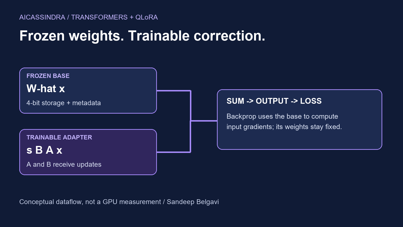
Use a column-vector convention for the equations. Let A have shape r by d and B have shape k by r, with r much smaller than the layer widths. Let W-hat denote the effective dequantized base weight used by the computation. A standard LoRA layer computes:
h = W-hat x + s B A x
W-hat: [k, d]    A: [r, d]    B: [k, r]
x: [d]          h: [k]       s = alpha / r
The first term supplies the pretrained transformation. The second supplies the learned correction. Standard LoRA scales it by alpha divided by rank; alternatives such as rank-stabilized LoRA use a different scaling rule. Always record the actual configuration. In the Python example below, inputs are row vectors, so transposes implement the same equation. PEFT documents the scaling and initialization options.
Quantized storage and arithmetic precision are separate choices. Four-bit codes plus metadata represent the base compactly; supported kernels reconstruct the values needed for computation. That does not mean every activation, gradient and multiplication is four-bit, or that a complete dequantized copy must remain resident throughout training.
Follow the gradient without changing the base
For a single example, write g for the loss derivative with respect to h and z = A x. Applying the chain rule to the displayed equation gives the following local derivatives. For a batch or sequence, contributions are summed or averaged according to the loss reduction:
dL/dB = s g z^T
dL/dA = s (B^T g) x^T
dL/dx = W-hat^T g + s A^T B^T g
These are algebraic derivatives of the simplified layer, not measured training results. The last line explains the apparent contradiction: W-hat participates in the input derivative even when no parameter gradient is accumulated for the base and no optimizer update is applied to it. Earlier trainable modules need that input derivative. The adapter can learn because its floating-point factors receive gradients; the packed base codes remain fixed.
For the intended adapter-only setup, construct the optimizer from the trainable parameters and inspect that list. Some configurations deliberately train extra modules or biases. Describe those exceptions explicitly rather than assuming that every parameter outside A and B is frozen.
Freezing is different from disabling autograd
Setting a parameter to requires_grad=False prevents accumulation of its own gradient. It does not prevent autograd from differentiating operations with respect to other inputs that require gradients. Wrapping a whole frozen forward branch in torch.no_grad() instead removes that branch from the recorded graph. These have different consequences when an earlier adapter needs a gradient through the frozen transformation. PyTorch explains this distinction in its autograd mechanics.
For example, an adapter near the beginning of a transformer can influence the input of a later frozen projection. If that later projection is evaluated without recording its input derivative, the earlier adapter loses part of its learning signal. Residual and parallel adapter paths may still produce a nonzero gradient, making the bug harder to spot. A nonzero gradient alone is insufficient; compare it with the expected path.
Run a small gradient check on synthetic tensors
Install PyTorch in an isolated environment, save this example as gradient_check.py, and run python gradient_check.py. It runs on the CPU, downloads no model and uses only the tensors shown here. It checks two backward passes, verifies the analytic input derivative and demonstrates the failure introduced by no_grad. This is an autograd illustration, not an NF4 implementation or a QLoRA benchmark.
# Author: Sandeep Belgavi. Synthetic CPU gradient check, not QLoRA training.
import torch

torch.manual_seed(7)
dtype = torch.float64
# A fixed floating-point stand-in for a dequantized base weight.
# No NF4 packing, CUDA, pretrained model or quantization kernel is used.
W = torch.tensor([[0.5, -0.25], [0.125, 0.75]], dtype=dtype)
A = torch.nn.Parameter(torch.randn(1, 2, dtype=dtype) * 0.1)
B = torch.nn.Parameter(torch.zeros(2, 1, dtype=dtype))
x = torch.tensor([[1.0, -2.0]], dtype=dtype, requires_grad=True)
target = torch.tensor([[0.0, 1.0]], dtype=dtype)
optimizer = torch.optim.SGD([A, B], lr=0.1)
original = W.clone()

for step in range(2):
    optimizer.zero_grad(set_to_none=True)
    x.grad = None
    y = x @ W.T + (x @ A.T) @ B.T  # scale = 1
    loss = ((y - target) ** 2).mean()
    loss.backward()
    # Two outputs: derivative of mean squared error is y - target.
    g = (y - target).detach()
    expected_dx = g @ W + (g @ B.detach()) @ A.detach()
    assert torch.allclose(x.grad, expected_dx)
    assert W.grad is None
    assert torch.equal(W, original)
    assert B.grad.norm().item() > 0
    if step == 0:
        assert A.grad.norm().item() == 0  # B initially zero
    else:
        assert A.grad.norm().item() > 0
    print(f"step={step} A_grad={A.grad.norm().item():.6f} "
          f"B_grad={B.grad.norm().item():.6f} base_unchanged=True")
    optimizer.step()

# A deliberately broken path: no_grad discards the base contribution to dx.
z = x.detach().clone().requires_grad_(True)
with torch.no_grad():
    base = z @ W.T
broken = base + (z @ A.detach().T) @ B.detach().T
broken.sum().backward()
correct_dx = torch.ones_like(broken) @ (W + B.detach() @ A.detach())
assert not torch.allclose(z.grad, correct_dx)
print("no_grad base branch: missing input gradient detected")
Expected behavior: the base stays identical, B receives a gradient on both steps, and A receives a zero gradient on the first step followed by a nonzero gradient on the second. With the common initialization of random A and zero B, the initial adapter contribution is zero; the first update to B opens the gradient path to A. The final assertion detects the missing base contribution in the deliberately broken branch. Exact printed magnitudes can depend on the installed PyTorch version; the assertions express the intended invariants.
Separate the memory savings from the remaining costs
The original QLoRA method uses NF4 weight storage, quantization of quantization constants, and paged optimizers to address memory pressure. Its published model-quality and hardware results belong to the authors' experiments; this article makes no matching-performance or device-fit claim. The local example above never executes these mechanisms. Read the original method and experimental conditions.
| Allocation | What to account for |
|---|---|
| Frozen base | Packed weights, scales, metadata and any unquantized modules |
| Adapter training | A and B, their gradients and optimizer-specific state |
| Execution | Saved activations, temporary buffers, kernels and allocator overhead |
| Other consumers | Runtime context, evaluation generation and competing processes |
For a hypothetical square layer of width 4,096 at rank 16, A and B contain 131,072 parameters, compared with 16,777,216 entries in the base matrix: 0.78125 percent. If those adapter parameters alone occupy two bytes each, their raw storage is 256 KiB. That excludes gradients, optimizer state and every other row of the table. A hypothetical seven-billion-parameter array at exactly four bits per entry occupies 3.5 GB, or about 3.26 GiB, before metadata and overhead. Neither calculation is a training-memory estimate.
The Transformers bitsandbytes guide separates the four-bit storage format from the compute dtype. Sequence length, microbatch size, checkpointing and the attention implementation can still determine whether a run fits. Measure the complete run instead of extrapolating from the adapter file size.
Map the explanation onto a real configuration
In the documented PEFT flow, load the supported model with a four-bit quantization configuration, prepare it for k-bit training, then attach adapters. Common configuration fields include load_in_4bit, bnb_4bit_quant_type, bnb_4bit_compute_dtype and bnb_4bit_use_double_quant. These select different aspects of representation and computation. Follow the official quantized-adapter preparation guide for the pinned library versions.
Choose target modules from the actual architecture. Query/value-only adaptation and adaptation of all supported linear layers are different experiments. Names such as q_proj are architecture-specific, and grouped-query attention can give key/value projections different output widths from query projections. Count each selected matrix with its real shape. The low-rank arithmetic remains valid for rectangular matrices.
Before a long run, inspect trainable parameter names, do one forward/backward step, check finite losses and intended gradients, and verify that the base parameters are unchanged. Save the base checkpoint identifier and revision with the adapter configuration. An adapter checkpoint alone does not normally contain a standalone base model.
Evaluate behavior before calling the adaptation useful
For a generic technical task, generate synthetic inputs such as short expressions with deterministic labels. Separate training and held-out templates before fitting. Compare the unchanged base and adapted model with the same prompt, decoding configuration and output validator. Report correctness, format validity and representative failures. A successful backward pass proves a gradient path, not improved generalization.
Record the model revision, software versions, quantization settings, target modules, rank, scaling, optimizer, sequence length and effective batch size. If reporting memory, distinguish peak allocated memory from reserved memory and process-wide device use. If reporting speed, state the workload and measurement boundaries. This article provides conceptual explanation, calculated parameter counts and a tiny synthetic check; it does not report language-model training, GPU measurements or quality improvements.