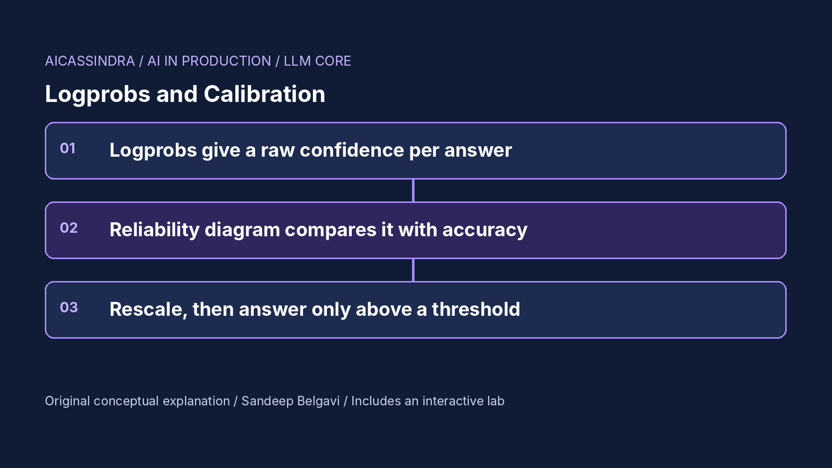
Every answer a language model produces comes with a by-product that most applications throw away: the log-probability of each generated token. Used well, it is the cheapest signal you have for deciding when a model is guessing, which matters for routing uncertain questions to a person, for refusing to auto-fill a field, or for deciding whether a classification can skip review. Used naively, it is a number between zero and one that says 0.97 on answers that are wrong a third of the time.
This guide covers what logprobs measure, how to check whether they are calibrated with reliability diagrams, expected calibration error, Brier score and AUROC, how temperature scaling and Platt scaling repair the numbers without changing the ranking, how to choose an abstention threshold from a risk-coverage curve, and why multi-token answers, chat tuning and domain shift break naive confidence. The lab scores 2,000 synthetic answers and lets you calibrate, threshold and stress them.
What a logprob is, and what it is not
For each generated token, the model's softmax assigns a probability; its natural logarithm is the logprob. For a single-token answer, such as a class label or a multiple-choice letter, exp(logprob) is the model's probability for that answer given the prompt. For a multi-token answer, the probability of the whole sequence is the product of the token probabilities, so its log is the sum of the token logprobs:
single token:   p("B")             = exp(-0.05)          = 0.951
sequence:       p("Rs 450, ships Monday") = exp(sum of 7 token logprobs)
                if every token has p = 0.97:  0.97^7 = 0.81
length-normalised (geometric mean per token): exp(mean logprob) = 0.97
Three cautions apply before you treat any of these as "the probability the answer is correct". First, the model's probability for a string is not the probability that the string is true; a model can be very sure of a wrong answer it has seen often. Second, many different strings can express the same answer, so the probability of one phrasing understates the model's belief in the answer. Third, the logprobs you receive may already be altered: by the sampling temperature, by penalties, or by whatever the provider exposes. Check whether your server reports log-probabilities from the raw distribution or after processing; this differs between systems and has changed between versions of some servers.
The OpenAI-compatible chat API returns per-token logprobs and optional top alternatives when you request them; vLLM supports logprobs for generated tokens and for the prompt; some hosted APIs do not expose them at all. Where they are unavailable, sampling-based confidence (agreement across several samples) is the usual substitute.
Calibration, measured four ways
A predictor is calibrated if, among all answers given with confidence c, a fraction c are correct. The standard picture is the reliability diagram: group answers into confidence bins, plot each bin's accuracy against its mean confidence, and compare with the diagonal. Bars below the diagonal mean overconfidence; above it, underconfidence.
| Metric | Definition | What it tells you |
|---|---|---|
| Expected calibration error (ECE) | Sum over bins of (bin share) × |mean confidence − accuracy| | Average gap between stated and actual reliability |
| Brier score | Mean of (confidence − outcome)², with outcome 0 or 1 | Calibration and sharpness together; lower is better |
| Negative log-likelihood | Mean of −log(confidence of the actual outcome) | Punishes confident mistakes hard; used to fit scaling |
| AUROC | Probability a random correct answer has higher confidence than a random wrong one | Ranking quality, independent of calibration |
Two of these measure different things and are worth keeping apart. AUROC is about ranking: can confidence separate right from wrong? ECE is about the numbers: does 0.8 mean 80%? A signal can rank perfectly and be badly miscalibrated (every correct answer at 0.99, every wrong one at 0.98), or be well calibrated and useless (every answer at the base accuracy). Selective answering needs good ranking; any downstream use that reads the number as a probability, such as expected-cost routing or showing confidence to users, needs good calibration as well.
ECE has known estimation problems. It depends on the number of bins, and with few examples in a bin the per-bin accuracy is noisy. Report the bin count, use at least a few hundred labelled examples, and prefer equal-mass bins if confidence is concentrated near one end. The lab lets you change the bin count and see how much ECE moves.
Why models are miscalibrated
Studies of large pretrained language models have found them reasonably well calibrated on multiple-choice questions when the format is right; Anthropic's work on whether models know what they know reported good calibration for larger models on many benchmarks. Two things commonly break it in production.
Post-training. Instruction tuning and preference optimisation reward confident, helpful answers. The GPT-4 technical report showed a calibration plot in which the pretrained model was well calibrated on a multiple-choice benchmark and the post-trained model noticeably less so. In practice chat-tuned models often put very high probability on their chosen answer token, which is what the lab's chat-tuned event models: the same underlying knowledge, sharpened log-odds, larger red gaps above the bars.
Distribution shift. Calibration is a property of a model on a distribution, not of the model alone. When traffic moves to topics, formats or languages where the model is less accurate, its confidence often does not fall with its accuracy. A calibration fit on last quarter's traffic can be badly off this quarter. The lab's new-domain event makes the model roughly 24 points less accurate on half the traffic (about 12 points overall) while its confidence stays where it was.
A third cause is the signal itself. For multi-token answers, raw sequence probability falls with length regardless of correctness, and length-normalised scores dilute the few tokens that carry the answer with many tokens that only carry phrasing. Methods that group samples by meaning, such as semantic entropy, exist precisely because token-level probabilities conflate "unsure what to say" with "unsure how to say it".
Repairing the numbers: temperature and Platt scaling
Temperature scaling, popularised for neural network classifiers by Guo and colleagues, fits one scalar T on a held-out labelled set and divides the log-odds (or logits) by it. Platt scaling fits a scale and an offset. For a binary "is this answer correct?" confidence c:
z = log(c / (1 - c))                 # log-odds of the raw confidence
temperature scaling:  c' = sigmoid(z / T)          # one parameter
Platt scaling:        c' = sigmoid(z / T + b)      # scale and bias

fit T (and b) by minimising negative log-likelihood on labelled examples
T > 1 softens overconfident scores; b < 0 shifts all scores down
Both are monotonic: they never change which answer is more confident than which, so AUROC and the ordering used by a threshold stay the same. They change what the numbers mean, which changes where the threshold must sit for a given target. This is also their limit. If the signal does not rank right above wrong, no rescaling helps; you need a better signal.
Temperature alone corrects stretch but not offset. When a model becomes wrong more often at every confidence level, as after a domain shift, the curve moves down rather than flattening, and only a bias term (or a richer method such as isotonic regression) moves it back. In the lab, temperature alone cannot bring calibration error under 5% on the shifted traffic; temperature plus bias can. A few hundred to a few thousand labelled examples are usually enough to fit two parameters stably, but they must come from the traffic you are calibrating for.
Answering only when sure: thresholds and risk-coverage
Selective prediction turns a confidence signal into a policy: answer when confidence is at least τ, otherwise abstain, ask a clarifying question or route to a fallback. The risk-coverage curve sorts answers by confidence and plots accuracy on the answered set against the share answered. Choosing τ means choosing a point on that curve.
With a calibrated signal the arithmetic is direct. If you answer only when calibrated confidence is at least 0.75, every answered item has an expected accuracy of at least 75% and the answered set's accuracy is the average of their confidences, typically well above τ. Expected wrong answers shipped per 1,000 questions is 1,000 × coverage × (1 − answered accuracy). In the lab's calibrated baseline, answering everything ships about 236 wrong answers per 1,000; a threshold of 0.75 answers 66% of questions at about 92% accuracy, shipping about 52.
Set τ from costs, not from habit. If a wrong answer costs ten times what a deferral costs, answer when expected loss from answering is lower: (1 − c) × 10 < 1, so c > 0.9. That calculation is only valid if c is calibrated, which is why calibration and abstention belong together. Mission two asks for at least 92% accuracy on answered questions while answering at least 60%; the window of thresholds that satisfies both is narrow, and the best answer is the lowest threshold that clears the accuracy bar.
Better signals for multi-token answers
When answers are free text, you have several confidence signals with different costs.
| Signal | Cost | Strength | Weakness |
|---|---|---|---|
| Sequence probability (sum of logprobs) | Free with logprobs | Exact model probability of that string | Falls with length; phrasing uncertainty dominates |
| Mean token logprob | Free with logprobs | Removes length bias | Dilutes the decisive tokens |
| Logprob of a short answer slot | Free, needs a structured format | Targets the decisive tokens | Requires the answer in a fixed position |
| Agreement across k samples | k extra generations | Measures consistency of the answer, works without logprobs | Coarse for small k; costs k times more |
| Verifier or P(True) prompt | One extra call | Can use reasoning about the answer | Needs its own calibration |
A cheap and often strong option is to restructure the output so the decisive information is a short field, such as a label, an ID or a yes/no, and read the logprob of that field. Self-consistency style agreement (sample several answers and measure how often they agree) needs no logprobs and handles paraphrase if you compare answers after normalisation or by meaning. Mission four reproduces the trade-off: with multi-token answers, sequence probability ranks poorly, mean logprob is close but not enough, and agreement across four samples clears the bar at five times the model cost.
A worked example: an order-status assistant
Consider a hypothetical Belgavi's Book Store assistant that answers order-status questions and hands uncertain ones to a support agent. The numbers below come from the lab's synthetic model, not from any deployment.
The team logs mean token logprob for each answer and labels 2,000 past answers. The raw scores say 0.9 for answers that are right much less often: expected calibration error is about 6 points for the base model and over 9 for the chat-tuned one. Fitting temperature on the labelled set gives T near 1.5 for the base model and near 2.1 for the chat-tuned model, bringing ECE to around 2 points or less. AUROC stays at about 0.88 throughout, because scaling does not change ranking.
With calibrated scores, a threshold of 0.75 sends about a third of questions to people and cuts wrong answers shipped from about 236 to about 52 per 1,000. Then a new product line launches, half the questions come from it, and the assistant's accuracy on those falls. Wrong answers shipped at the old settings more than double, to about 110 per 1,000, while the dashboard's confidence numbers look unchanged. Refitting on a fresh labelled sample needs a bias term (b near −1), after which a threshold of 0.8 ships about 30 wrong answers per 1,000 at roughly 41% coverage. The lesson is the procedure: label a fresh sample regularly, refit, and re-derive the threshold from costs.
Detecting calibration drift and common mistakes
Calibration fails quietly, so monitor it explicitly.
- Keep a labelled stream. Sample a small fixed share of answered and abstained items for human labelling every week. Abstained items matter: without them you cannot see whether the threshold is too strict.
- Track ECE, AUROC and answered accuracy by segment: product area, language, prompt version and model version. A global number hides a shifted segment.
- Watch the confidence distribution. A shift in the histogram of confidence, with no change in labelled accuracy yet, is an early warning that inputs have changed.
- Refit on every model or prompt change. A new model version, a new system prompt or a change of sampling temperature invalidates the old fit.
Common mistakes: treating raw sequence probability as a confidence for free text; reading logprobs from a sampled answer at high temperature and assuming they reflect the model's base distribution; reporting ECE without the bin count or sample size; setting a threshold on uncalibrated scores and then reading it as a probability; and calibrating on a benchmark rather than on your own traffic.
The lab follows the same sequence: fix a chat-tuned model's overconfidence, choose an abstention threshold, recover from a domain shift that needs a bias term, and pick a confidence signal for multi-token answers within a cost budget.
Run the lab: Calibration lab: make 90% confident mean 90% right
The lab generates 2,000 synthetic questions of varying difficulty, decides whether a simulated model answers each correctly, and gives each answer a confidence from the signal you choose. The left panel is a reliability diagram: blue bars are accuracy per confidence bin, red shading is overconfidence, green is underconfidence, and teal bars underneath show how many answers fall in each bin. The right panel is the risk-coverage curve, with your abstention threshold marked in yellow. Start with raw scores, read the insight for the best-fitting temperature, then load mission one.
Prefer a full-width view? Open the standalone lab. Your stars are saved in this browser and shown on the series hub.
What to do next
- Check whether your provider or server returns logprobs, and whether they are raw or after temperature and penalties.
- Label 500 to 2,000 recent answers and draw a reliability diagram with ECE, Brier score and AUROC, stating the bin count.
- Fit temperature, and a bias term if needed, on that labelled set; refit whenever the model, prompt or sampling settings change.
- Choose an abstention threshold from the cost of a wrong answer versus a deferral, using calibrated scores.
- For free-text answers, move the decisive information into a short field or use agreement across samples instead of raw sequence probability.
- Set up a weekly labelled sample, including abstained items, and track calibration by segment.
Sources and further reading
- Guo et al., On Calibration of Modern Neural Networks (ICML 2017)
- Kadavath et al., Language Models (Mostly) Know What They Know
- OpenAI, GPT-4 Technical Report (calibration before and after post-training)
- Kuhn, Gal and Farquhar, Semantic Uncertainty: Linguistic Invariances for Uncertainty Estimation in Natural Language Generation (ICLR 2023)
- Wang et al., Self-Consistency Improves Chain of Thought Reasoning in Language Models (ICLR 2023)
- Geifman and El-Yaniv, Selective Classification for Deep Neural Networks (NeurIPS 2017)
Related in this series:
- Sampling Settings That Fix Real Failures: Temperature, Top-p and Min-p
- Constrained Decoding: How JSON Schema Mode Masks Invalid Tokens
- Tokenizers Decide Your Bill: How BPE Merges Treat Languages and Code
Diagrams, examples and the lab model are original educational material. Lab numbers are calculated by a synthetic model, not measured on real hardware or services.
Views are my own and do not represent any employer, past or present.