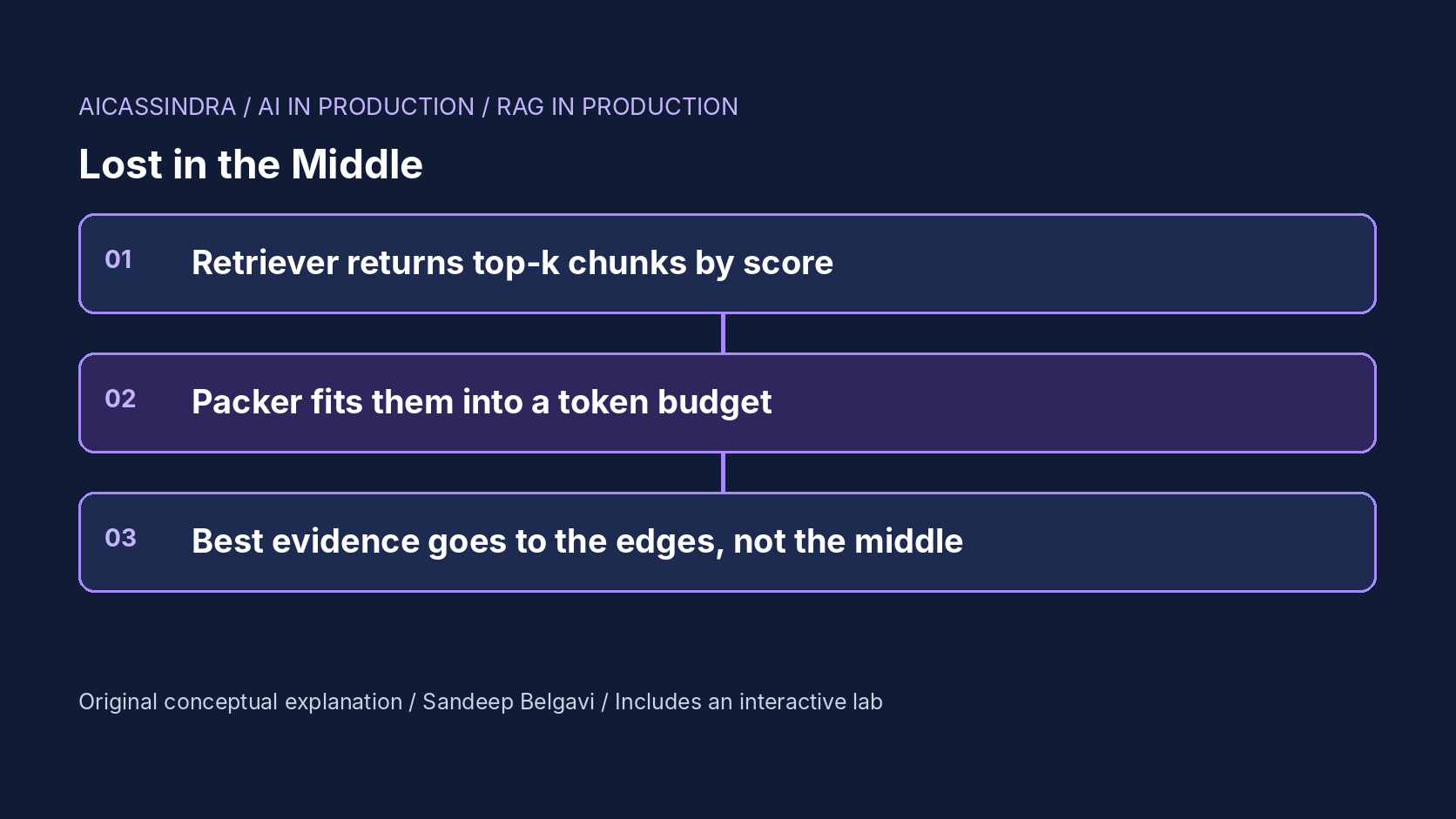
A retrieval-augmented system can find the right passage and still answer wrong. The retriever did its job, the passage is in the prompt, and the model answers from a different chunk, from its own memory, or not at all. One of the most reproducible reasons is position: long-context models use information near the start and the end of the prompt more reliably than information in the middle. Stuff twenty chunks into a prompt in arbitrary order and a good share of your answers land exactly where the model looks least.
This guide covers what the positional effect is and why it appears, the arithmetic of how chunk count, chunk size and ordering decide where the answer lands, how to pack chunks under a token budget (deduplication, per-document caps, neighbour expansion), the knobs that exist in common RAG frameworks, and how to measure the effect on your own traffic instead of trusting a benchmark. The embedded lab lets you retrieve, pack and order synthetic chunks and see expected accuracy, prompt tokens and cost move together.
What the positional effect is
The effect has a name because of a 2023 paper, Lost in the Middle: How Language Models Use Long Contexts (Liu et al., later published in TACL). The setup was simple: multi-document question answering where exactly one of 10, 20 or 30 retrieved documents contains the answer, and the position of that document is varied. Accuracy traced a U-shape. It was highest when the answer document came first or last and lowest when it sat in the middle, and for some models in the 20-document setting the middle positions scored at or below the accuracy of answering with no documents at all. Models marketed with longer context windows were not reliably better at using the middle of what they were given.
Later benchmarks such as RULER made the same point from another angle: the context length a model accepts and the length it can use well are different numbers, and the gap depends on the task. Newer models have narrowed the dip on simple retrieval tests, so treat the size of the effect as something to measure for your model, not a constant. What has stayed true across model generations is the shape: when evidence is buried in a long block of similar-looking text, the edges are the safest places to put it.
There are several plausible contributors. Causal attention means early tokens are visible to every later position, and models learn to lean on the start of the sequence (the so-called attention sink behaviour). Recency helps the end: tokens close to the question and the generation point are cheap to attend to. And training data rarely rewards fetching one fact from the exact middle of 20,000 tokens of near-duplicates. None of these is fully settled, but you do not need the cause to engineer around the symptom.
The arithmetic of where the answer lands
Model the probability that the model uses a piece of evidence as a function of its relative position x in the prompt, from 0 (start) to 1 (end). The lab uses an illustrative curve: accuracy at the edges minus a dip that is zero at both ends and maximal at x = 0.5, with a depth that grows with prompt length. The exact numbers are calculated, not measured, but the reasoning carries over.
P(correct | answer at x) = edge - depth(T) * bump(x) - distractor_penalty
bump(x)   = 1 - |2x - 1|^1.6          # 0 at the edges, 1 in the middle
depth(T)  = 0.40 * clamp(log2(T / 1500) / 4, 0, 1)

T =  3,552 tokens -> depth = 0.12   (12 points at the middle)
T =  8,336 tokens -> depth = 0.25
T = 24,000 tokens -> depth = 0.40   (saturated)
Now ask where the answer lands under each ordering. In source order (concatenated by document id or ingestion time), the answer chunk's position is effectively uniform. The average of bump(x) over a uniform x is 1 - 1/2.6, about 0.62, so you lose about 62% of the full dip on average, roughly 15 points at 8,000 tokens. About a third of answers land in the middle third, where the loss is close to the full 25 points.
With the chunks sorted by retriever score, best first, the answer is usually rank 1 or 2 and lands at x near 0.05 to 0.1, where bump is small. The residual loss comes from queries where the retriever ranked the answer fifth or tenth. An edges-first ordering (rank 1 at the start, rank 2 at the end, rank 3 second, rank 4 second-to-last, and so on) protects ranks 1 and 2 and pushes the weakest chunks to the middle, where being ignored costs nothing. With 20 chunks, the lab's model gives about 68% expected accuracy in source order, about 75% best first, and about 77% edges first. The gap between best first and edges first is small when the retriever is sharp and grows when the answer is often at rank 2 to 4.
The second lever is T itself. Each halving of prompt length lowers log2(T) by one, which in this curve removes 0.25 × 0.40 = 0.10, about 10 points of dip below the saturation point, while also halving input cost and roughly halving prefill time. Ordering protects the evidence you have; shortening the prompt makes the whole curve flatter.
Ordering strategies compared
There are four orderings you will meet in practice, and it is worth knowing why each exists.
| Ordering | Where rank 1 lands | Strength | Weakness |
|---|---|---|---|
| Source order (doc id, time) | Anywhere | Preserves narrative order inside a document | Answer lands mid-prompt about a third of the time |
| Best first | Start | Simple; strong when rank 1 is usually right | Rank 2 to 4 drift toward the middle in long prompts |
| Best last | End, next to the question | Uses recency; good for short prompts | Weak chunks occupy the start, which models also favour |
| Edges first (alternating) | Start, rank 2 at the end | Top evidence avoids the dip; weak chunks absorb it | Breaks reading order across chunks of one document |
The reordering is a few lines of code. The version below is the alternating scheme that LangChain and LlamaIndex both ship under the name LongContextReorder (check your version's documentation for the exact import path and whether it expects ascending or descending input):
def edges_first(chunks):
    """chunks sorted by relevance, best first -> best at both ends, weakest in the middle"""
    head, tail = [], []
    for i, c in enumerate(chunks):
        (head if i % 2 == 0 else tail).append(c)
    return head + tail[::-1]

# ranks 1..6 -> positions: [1, 3, 5, 6, 4, 2]
One subtlety: when several chunks come from the same document, it often helps to keep them adjacent and in their original order, then order the groups by their best chunk score. A table split into three chunks is much easier to read in sequence than scattered across the prompt. And whatever order you pick, keep the instructions and the question in fixed places: long documents first and the question at the end is a common recommendation in model vendors' long-context guides.
Packing under a token budget
Ordering assumes you already know which chunks go in. Packing is the step that decides that, and it fails more quietly. A packer takes the ranked list, a token budget and some rules, and emits the final context. The rules that matter most:
- Count tokens with the real tokenizer. Character or word estimates drift by 20% or more on code, tables and non-English text, and an overflowing prompt gets truncated by the server or the client, usually from the end, which is exactly where you put rank 2.
- Deduplicate before you cut to top-k. Re-crawled pages, mirrored documentation and boilerplate sections produce near-identical chunks with near-identical scores. They arrive adjacent in the ranking and each one takes a slot that a different piece of evidence could have used. Hash normalised text for exact copies and use a similarity threshold (for example cosine above about 0.95, tuned on your data) for near copies, and over-fetch so that dropping copies still leaves k chunks.
- Cap chunks per document. One long, highly similar document can take every slot; a cap of two or three per source keeps diversity. Maximal marginal relevance (MMR) does the same thing more smoothly.
- Expand neighbours when the answer is split. Small chunks retrieve precisely but cut facts in half. Fetching the previous and next chunk of a high-scoring hit restores context without retrieving more noise.
def pack(ranked, budget, tok, per_doc_cap=3, sim_dup=0.95):
    out, used, per_doc = [], OVERHEAD_TOKENS, {}
    for c in ranked:                                   # best first, over-fetched (e.g. 3x k)
        if any(cosine(c.vec, o.vec) > sim_dup for o in out):
            continue                                   # near-duplicate of something kept
        if per_doc.get(c.doc_id, 0) >= per_doc_cap:
            continue
        n = tok(c.text)
        if used + n > budget:
            continue                                   # skip, a smaller chunk may still fit
        out.append(c); used += n; per_doc[c.doc_id] = per_doc.get(c.doc_id, 0) + 1
        if len(out) == K:
            break
    return edges_first(out), used
Note the order of operations: filter, then pack, then reorder. Reordering before packing lets the budget cut chunks by position instead of by relevance.
Chunk size, top-k and the cost of a long prompt
The positional dip makes top-k and chunk size more expensive than they look. Every extra chunk adds tokens (cost and prefill time), deepens the middle dip and adds a distractor that can mislead the model. The benefit is only recall: a better chance that the answer is somewhere in the prompt. Past the point where recall saturates, more context is pure loss.
Chunk size pulls in two directions. Smaller chunks give sharper embeddings, so the answer chunk ranks higher, and they let you fit more distinct sources into the same budget. But if a fact spans about 40 tokens and its start is uniformly placed, the chance it straddles a chunk boundary is roughly 40 divided by the chunk size: 40% at 100 tokens, 13% at 300, 7% at 600. A split answer gives the model half the evidence. The lab models both effects; in its synthetic world the sweet spot sits around 150 to 200 tokens with 6 to 10 chunks, but the location of that sweet spot depends entirely on your documents.
Prefill time also scales with prompt length. As an illustrative rule, if a serving stack prefills around 20,000 tokens per second for one request, a 2,000-token prompt adds about 100 ms before the first token and a 20,000-token prompt adds about a second, before any queueing. Prefix caching (for example vLLM's automatic prefix caching; check your version's flag and default) helps only for the shared prefix, which is the system prompt, not the retrieved chunks that differ per query.
A worked example: Belgavi's Book Store
Suppose the hypothetical Belgavi's Book Store runs a support assistant over its policy pages, catalogue notes and order FAQs. The first version retrieves the top 30 chunks of 600 tokens each and concatenates them in document-id order. Here are the lab's calculated numbers for that setup and three fixes, at an illustrative input price of $3 per million tokens:
| Setup | Prompt tokens | Expected accuracy | Input cost per 1k queries |
|---|---|---|---|
| k = 30, 600-token chunks, edges first | about 18,300 | 75% | $55 |
| k = 20, 400-token chunks, source order | about 8,300 | 68% | $25 |
| k = 20, 400-token chunks, edges first | about 8,300 | 77% | $25 |
| k = 8, 150-token chunks, edges first, deduplicated | about 1,550 | 80% | $4.70 |
Two things stand out. Reordering the same 20 chunks is worth about nine points for free. And the cheapest setup is also the most accurate one, because the answer chunk ranks higher with smaller chunks, the prompt is short enough that the dip is shallow, and there are fewer hard negatives to confuse the model. At a million queries a month, the difference between the first and last rows is about $50,000 in input tokens alone. All these numbers come from a synthetic model; the procedure, not the values, is what transfers: measure recall at each k, find where it flattens, and buy no more context than that.
Detecting position problems in production
Position effects hide in aggregate metrics. Overall accuracy can look stable while one slice, such as long questions that retrieve many chunks, degrades. The useful signals are cheap to log:
- The rank and position of the cited chunk. If your system asks for citations, log which chunk each answer cited and where it sat in the prompt. A histogram of cited positions that is heavy at the edges and empty in the middle, while the retriever's ranks are spread out, is the dip showing up in your own traffic.
- A position-swap evaluation. Take a labelled set where you know the answer chunk, and run each question several times with the answer chunk moved to the start, the middle and the end. The accuracy gap between those runs is your model's dip at your prompt length. Re-run it whenever you change models; the dip is a property of the model.
- Prompt length percentiles. Track p50 and p95 of retrieved-context tokens per route. A packer change or a new document type that doubles chunk length moves the whole curve.
- Duplicate rate in packed context. The share of packed chunks that are near-copies of another packed chunk. It should be close to zero; a jump usually means an ingestion job re-indexed content without deleting the old version.
When accuracy drops, check whether the answer chunk was in the prompt before blaming position. If it was absent, it is a retrieval or packing problem. If it was present and not used, check where it was.
Playing the lab
The lab turns these rules into four puzzles. Mission one gives you twenty chunks in source order and asks for better accuracy without changing top-k or the budget; the only lever left is ordering. Mission two asks you to survive a duplicate flood, where re-crawled copies take top-k slots and push the answer out of the prompt entirely, with the chunk size fixed because re-indexing is not an option on the day. Mission three is the cost-versus-quality trade: someone set top-k to 30 and you need higher accuracy at a fraction of the input cost. Mission four combines retriever drift with a cheaper model that has a deeper middle dip, so you need more depth from retrieval while keeping the prompt short enough that ordering still works. Watch the bar chart under the prompt: it shows expected accuracy by where the answer chunk landed, which is the same position-stratified view you should build on your own evaluation set.
Common mistakes
The most common mistake is treating the context window as free capacity: if the model accepts 128,000 tokens, why not send 40 chunks? The answer is cost, latency, and a deeper middle dip, all to buy recall you could get from a better retriever or a reranker. The second is reordering by score after a fusion or reranking step without checking which score you sorted on; sorting on the first-stage similarity after a cross-encoder rerank throws the rerank away. Third, truncating an overflowing prompt from the end silently removes whatever was placed there, which in an edges-first layout is your second-best chunk. Fourth, evaluating with short prompts and deploying with long ones: an offline set with five chunks per question will not show a dip that your production prompts at 15,000 tokens have. Finally, assuming the dip is fixed. Model updates change it, sometimes a lot, so the position-swap test belongs in the regression suite that runs before every model change.
Run the lab: Lost in the middle: pack and order chunks so the answer gets read
The lab below generates 300 synthetic questions, each with one answer chunk, four hard negatives and many weaker chunks with retriever scores. Your controls retrieve the top k, deduplicate, pack into the context budget and order the result. The strip at the top shows one packed prompt (green is the answer chunk, pink hard negatives, orange duplicates, purple the question), the curve under it shows the positional dip at that prompt length, and the bars show expected accuracy by where the answer landed. Start with mission one and change only the ordering.
Prefer a full-width view? Open the standalone lab. Your stars are saved in this browser and shown on the series hub.
What to do next
- Log the prompt position and retriever rank of every chunk your answers cite, and plot cited positions against retrieved positions for a week of traffic.
- Build a position-swap evaluation: move the known answer chunk to the start, middle and end of the prompt and record the accuracy gap for your current model.
- Switch to an edges-first or best-first order and make sure the sort uses the final (reranked) score.
- Add deduplication with over-fetching before top-k, and alert on the share of near-duplicate chunks in packed context.
- Sweep top-k on your evaluation set, find where recall flattens, and cut k and the context budget to that point.
- Count tokens with the production tokenizer and make overflow drop the lowest-ranked chunk, never the last one in the prompt.
Sources and further reading
- Lost in the Middle: How Language Models Use Long Contexts (Liu et al., TACL 2024)
- RULER: What's the Real Context Size of Your Long-Context Language Models? (Hsieh et al., 2024)
- LangChain how-to: reorder retrieved results to mitigate the lost in the middle effect
- LlamaIndex example: LongContextReorder node postprocessor
- Anthropic documentation: long context prompting tips
Related in this series:
- Cross-Encoder Reranking Depth: How Many Candidates Are Worth the Latency
- Chunking Strategies Compared: Fixed, Recursive, Semantic and Late Chunking
- RAG Latency Budget: Where the Milliseconds Go Between Query and Answer
Diagrams, examples and the lab model are original educational material. Lab numbers are calculated by a synthetic model, not measured on real hardware or services.
Views are my own and do not represent any employer, past or present.