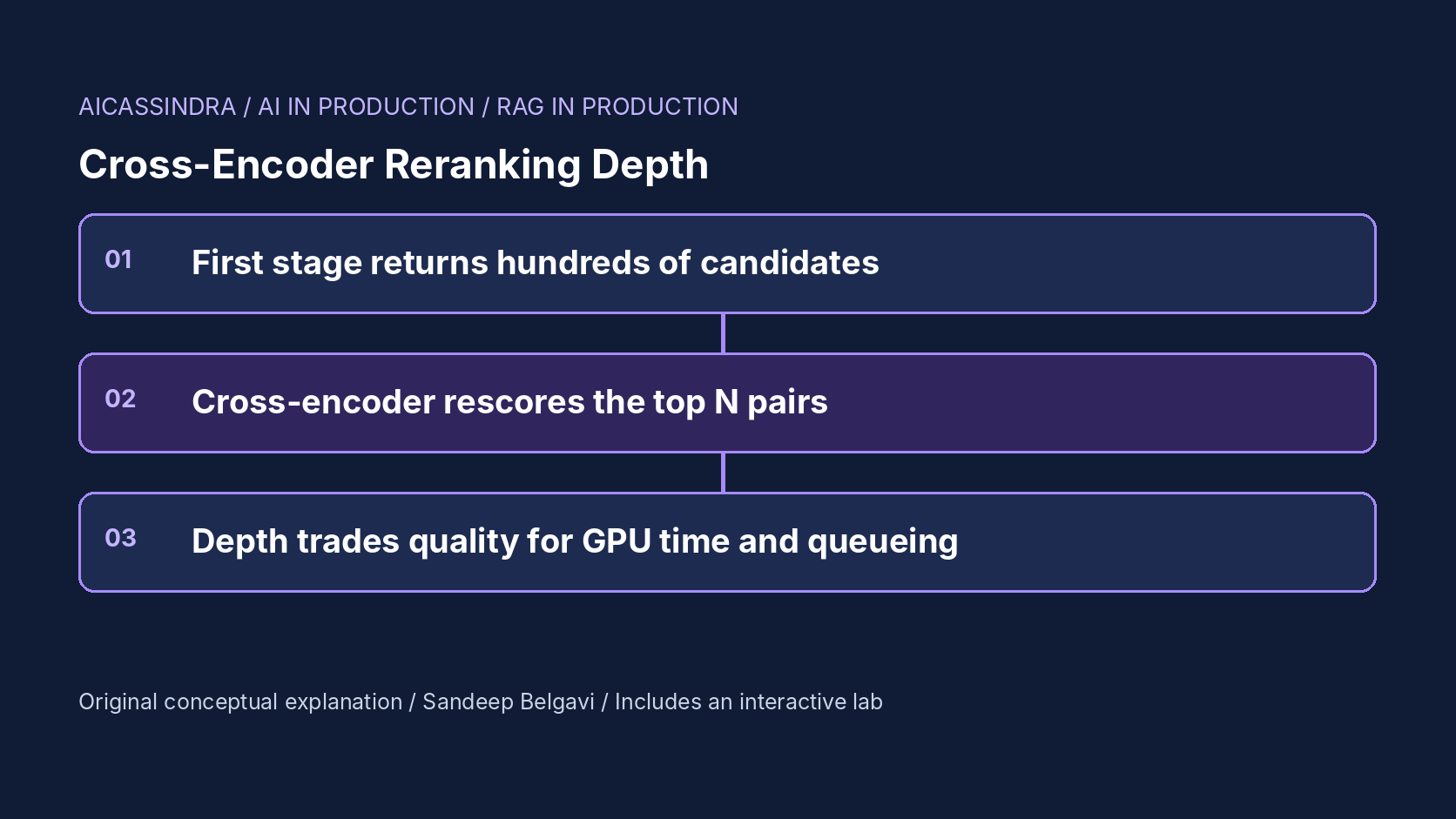
Adding a cross-encoder reranker is one of the most reliable quality upgrades in a RAG pipeline: the first-stage retriever finds plausible candidates quickly, and a model that reads the query and each passage together puts the right ones on top. The question every team then argues about is how many candidates to rerank. Twenty feels cheap and leaves quality on the table; two hundred feels thorough and quietly turns a 40 ms step into a queue that melts under the first traffic spike.
This guide works through the depth decision from first principles: why the first stage sets a ceiling the reranker cannot exceed, why quality gains flatten, what one query-passage pair costs on a GPU, and why latency is a queueing problem rather than a per-request one. It covers the knobs in common serving stacks and a procedure for choosing depth. The embedded lab reranks synthetic candidate lists and runs a GPU queue, so you can see the knee in the quality curve and the cliff in the latency curve at the same time.
Two stages, two kinds of model
First-stage retrievers, whether BM25, a bi-encoder embedding model or a hybrid, score a query against millions of documents by comparing precomputed representations. That is what makes them fast, and also what limits them: the document vector was computed without seeing the query, so fine distinctions such as negation, which product version a passage applies to, or whether it actually answers the question get blurred. A cross-encoder concatenates the query and one passage, runs a full transformer over the pair with attention across both, and outputs a relevance score. It is far more accurate per pair and far too slow to run against the whole corpus, so it runs on the first stage's top N.
Two facts follow and drive everything else. The reranker can only reorder what it is given, so the first stage's recall at depth N is a hard ceiling on what reranking can achieve. And the reranker's cost is linear in N for every single query, because each candidate is a separate forward pass (batched, but not shared). The original BERT passage reranking work on MS MARCO showed large gains from this architecture, and late-interaction models such as ColBERT were designed precisely to recover some of that accuracy at a fraction of the per-pair cost.
The recall ceiling and diminishing returns
Quality as a function of depth is the product of two curves. The first is the share of relevant passages the first stage places within the top N, which rises quickly and then slowly: most relevant passages sit near the top, a long tail sits deep. The second is how well the reranker sorts what it sees, which degrades a little as N grows, because deeper candidates include more hard negatives that look relevant. Multiply them and you get a curve with a knee.
| Depth (lab, base model, calculated) | Relevant inside depth | nDCG@5 | p95 rerank latency at 8 qps |
|---|---|---|---|
| 0 (no reranker) | 59% | 0.562 | 0 ms |
| 10 | 67% | 0.750 | 16 ms |
| 20 | 76% | 0.818 | 32 ms |
| 30 | 81% | 0.848 | 49 ms |
| 50 | 86% | 0.875 | 88 ms |
| 100 | 92% | 0.920 | 328 ms |
The first ten candidates buy about 0.19 of nDCG@5; going from 50 to 100 buys 0.045 for twice the compute and almost four times the p95. Where the knee sits depends on your first stage: a strong hybrid retriever puts relevant passages high, so shallow reranking captures most of the gain, while a weak or out-of-domain first stage pushes them deep and moves the knee to the right. With the lab's weaker first stage, depth 20 captures only 49% of relevant passages and nDCG@5 stays near 0.56 with the base model; reaching 0.70 takes a depth between 50 and 100. That is the strongest argument for improving the first stage before buying a bigger reranker.
What one pair costs
A transformer forward pass costs roughly 2 × parameters × tokens floating-point operations, counting only the parameters that do per-token compute. That last clause matters for multilingual rerankers, whose large vocabulary embedding tables hold a big share of the parameters but cost almost nothing to apply. A pair is the query plus the passage, so passage length enters linearly:
# per-pair compute, illustrative, non-embedding parameters only
base reranker  : ~86M compute params x 288 tokens x 2  = ~50 GFLOP per pair
large reranker : ~300M compute params x 288 tokens x 2 = ~173 GFLOP per pair

# a GPU sustaining ~65 TFLOPS on this workload
base  : 65e12 / 50e9  = ~1,300 pairs/s  -> depth 50 = ~38 ms of GPU time per query
large : 65e12 / 173e9 = ~380 pairs/s   -> depth 50 = ~130 ms of GPU time per query

# double the passage length and every number above doubles
The lab uses throughputs of this order (about 4,200, 1,300 and 420 pairs per second at 256-token passages for its small, base and large models). They are illustrative; real throughput depends on the GPU, precision, batch size, sequence padding and the serving stack, so measure your own. The structure, though, is fixed: cost per query is depth times tokens per pair times model size, and a chunking change that doubles passage length doubles reranking cost without anyone touching the reranker.
Latency is a queueing problem
Teams usually estimate reranking latency as service time: depth times time per pair. That is the latency of an idle GPU. In production the reranker is a shared server, and once utilization climbs, waiting time dominates. With arrival rate λ, service time S and c GPUs, utilization is ρ = λ × S / c. As ρ approaches 1, the queue grows without bound; in M/G/1-style models the mean wait scales with ρ / (1 - ρ), so going from 50% to 90% utilization multiplies waiting time by about nine.
In the lab, the base model at depth 50 has a service time of about 41 ms. At 8 queries per second on one GPU, utilization is about 33% and p95 is 88 ms. Triple the traffic and utilization reaches about 74%: p95 jumps to roughly 230 ms with nothing else changed, and depth 100 under the same surge saturates the GPU completely, with p95 measured in tens of seconds. A depth that is comfortable on an average afternoon can be the cause of an outage during a launch. That is why depth should be chosen against peak load with headroom, and why the safest emergency lever during a surge is to reduce depth or switch to a smaller reranker automatically, not to wait for autoscaling.
The knobs in real stacks
| Knob | Where it appears | Effect |
|---|---|---|
| Depth (top N) | Your retrieval code; framework reranker wrappers often call it top_n or similar | Linear cost, recall ceiling |
| Model | Sentence Transformers CrossEncoder; Hugging Face Text Embeddings Inference serving reranker models; hosted rerank APIs | Accuracy versus cost per pair |
| Max sequence length | max_length on the cross-encoder, server truncation settings | Caps tokens per pair; truncation can cut the answer |
| Batch size | batch_size in predict, server batching limits | Throughput versus per-request latency |
| Precision | fp16 or bf16 inference, ONNX or other optimized runtimes | Throughput, small accuracy changes |
Names and defaults differ by library and version, so check the documentation for the release you run. A minimal reranking step with Sentence Transformers looks like this:
from sentence_transformers import CrossEncoder

reranker = CrossEncoder("your-reranker-model", max_length=384)   # pick and pin a model

def rerank(query, candidates, depth=30, final_k=5):
    head = candidates[:depth]                     # first-stage order
    scores = reranker.predict([(query, c.text) for c in head], batch_size=32)
    order = sorted(zip(scores, head), key=lambda x: -x[0])
    return [c for _, c in order][:final_k]
Two details are easy to miss. Truncation at max_length silently cuts long passages, so the sentence that answers the question may never be scored; align the reranker's length limit with your chunk size. And scores from different queries are not calibrated probabilities, so a fixed score cut-off behaves differently across query types; use rank-based cut-offs unless you have calibrated them.
Choosing depth: a procedure
- Label a few hundred real queries with relevant passages (graded if possible) and log the first stage's top 200 for each.
- Compute the first stage's recall at 10, 20, 50, 100 and 200. This is the ceiling curve; if recall@50 is low, fix retrieval first.
- Rerank offline at each depth with each candidate model and compute nDCG@k or answer accuracy at the k you actually send to the LLM.
- Measure throughput in pairs per second for each model on your hardware at your passage length, and convert depth into service time.
- Pick the smallest depth within a small margin of the best quality, then check utilization at peak traffic. Keep peak utilization well below saturation, and define a degraded mode (smaller depth or model) for surges.
For the hypothetical Belgavi's Book Store assistant, suppose peak traffic is 20 queries per second and the base reranker's knee is near depth 30, with about 25 ms of GPU time per query. One GPU would run at about 50% utilization at peak, with p95 comfortably under 100 ms in the lab's model; depth 100 would need about four GPUs for the same headroom and would buy roughly 0.07 of nDCG@5. Spending that budget on a better first stage usually moves the whole curve up instead. These figures are calculated from the lab's illustrative assumptions, not measured.
Cheaper ways to buy the same quality
Depth is not the only lever, and several alternatives change the shape of the trade-off rather than sliding along it. A reranking cascade runs a small cross-encoder over a deep list, say the top 100, and a large one over the small model's top 20. Most of the compute goes to the cheap model, while the expensive model only judges candidates that already look good. Late-interaction models such as ColBERT precompute per-token document vectors and compare them with query token vectors at search time, which recovers much of a cross-encoder's precision at a cost closer to a bi-encoder's, at the price of much larger indexes. LLM-based rerankers that read several passages at once can be more accurate still, but their cost per query is higher again, so they usually sit behind a cross-encoder and see only a handful of candidates.
Two cheaper tricks are worth checking first. Caching rerank scores keyed by query and passage identifiers pays off for popular repeated questions. Adaptive depth reranks fewer candidates when the first stage is confident, for example when the top score is far above the rest or when the query is an exact identifier lookup that BM25 already answered, and more when the scores are flat. Both reduce average cost; neither removes the need to size for peak load.
Measuring quality where it matters
Rerankers are usually evaluated with nDCG or MRR at 10, but a RAG system cares about the k passages that actually reach the prompt, often three to eight. Evaluate at that k, and if possible measure answer correctness or citation accuracy downstream as well, because a reranker that moves the right passage from rank 6 to rank 4 is worth a lot when k is 5 and nothing when k is 10. Keep a held-out set from recent traffic, since a reranker tuned on last year's questions can drift quietly as the product changes. Finally, look at per-class results: rerankers can be strong on natural-language questions and weak on identifiers, tables or numeric comparisons.
Failure modes and common mistakes
- Depth set at an idle-GPU benchmark. Detect it by alerting on reranker queue time and GPU utilization, not only on service time.
- Chunking changes that double cost. Longer passages mean more tokens per pair; tie chunk-size changes to a reranker capacity check.
- Truncated passages. If chunks exceed the reranker's maximum length, the end of each passage is never scored; track the share of truncated pairs.
- Reranking too few after a first-stage regression. A new embedding model or index change can push relevant passages deeper; monitor first-stage recall at your depth on a labelled set.
- Bigger model as the default fix. A large reranker at shallow depth can lose to a small one at a sensible depth, and costs more.
The lab's missions follow these decisions. Mission one turns the reranker on and rewards the smallest depth that reaches the quality target within 60 ms. Mission two is a traffic surge on a large model that saturates two GPUs; the best answer meets the target on one GPU with a smaller model and a moderate depth. Mission three weakens the first stage so relevant passages sink, and asks you to go deeper without breaking the latency budget, which favours a smaller model. Mission four doubles passage length under a cost cap and asks you to find the model and depth that still fit.
Run the lab: Rerank depth: find the knee before the GPU queue finds you
The lab below generates first-stage candidate lists for synthetic queries with graded relevant passages and many hard negatives, reranks the top N with a simulated cross-encoder whose accuracy depends on model size, and runs a multi-GPU queue for the reranking work. On the left, the first-stage top 20 and the reranked top 20 show relevant passages in green moving up past the dashed top-5 line. On the right, nDCG@5 and p95 latency are plotted for every depth so you can see the knee and the cliff together. Start by changing the depth, then inject a traffic surge.
Prefer a full-width view? Open the standalone lab. Your stars are saved in this browser and shown on the series hub.
What to do next
- Measure first-stage recall at 10, 20, 50, 100 and 200 on labelled queries to find the ceiling your reranker works under.
- Sweep rerank depth offline and plot nDCG@k (at the k you send to the LLM) against depth for each candidate model.
- Benchmark reranker throughput in pairs per second at your real passage length, precision and batch size.
- Size reranker GPUs for peak traffic with utilization well below saturation, and alert on queue time and utilization.
- Align the reranker's maximum sequence length with your chunk size and track the share of truncated pairs.
- Define a degraded mode (smaller depth or model) that switches on automatically when reranker queue time rises.
Sources and further reading
- Passage Re-ranking with BERT (Nogueira and Cho, 2019)
- MS MARCO: A Human Generated MAchine Reading COmprehension Dataset
- ColBERT: Efficient and Effective Passage Search via Contextualized Late Interaction over BERT (SIGIR 2020)
- Sentence-BERT: Sentence Embeddings using Siamese BERT-Networks (EMNLP 2019)
- Hugging Face Text Embeddings Inference documentation
Related in this series:
- Reciprocal Rank Fusion Tuning: When BM25 Rescues Dense Retrieval Misses
- RAG Latency Budget: Where the Milliseconds Go Between Query and Answer
- Lost in the Middle: Ordering and Packing Retrieved Context for Long Prompts
Diagrams, examples and the lab model are original educational material. Lab numbers are calculated by a synthetic model, not measured on real hardware or services.
Views are my own and do not represent any employer, past or present.