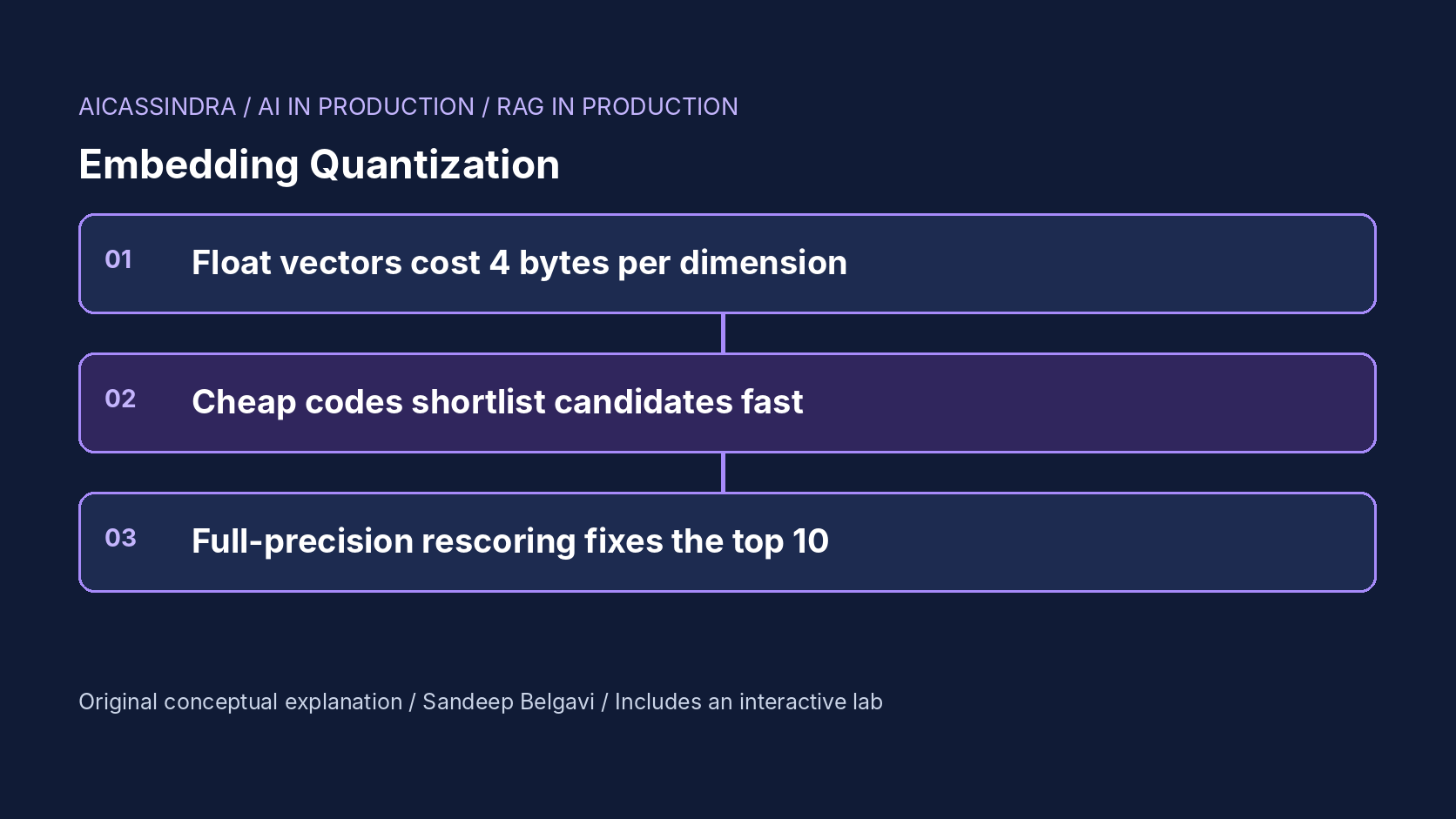
A vector index looks cheap until you multiply. One 1024-dimensional float32 embedding is 4 KB. A hundred million of them is about 410 GB before the graph links, and approximate nearest-neighbour search only stays fast while the vectors it touches live in RAM. Teams usually find this out when a new document source lands, the index outgrows its nodes, and p95 latency jumps from a few milliseconds to a few hundred because every graph hop is now a page fault.
Embedding quantization is the standard answer: store each dimension in one byte, half a byte or a single bit, and accept a small error in every similarity score. This guide works through what each encoding costs and loses, with the actual arithmetic; why rare outlier values and non-centred embedding models break quantizers in production; how oversampling and rescoring recover recall; and which knobs Qdrant, pgvector, Elasticsearch, FAISS and Sentence Transformers expose. The embedded lab lets you quantize a synthetic index and watch the true top 10 survive or fall apart.
What the bytes buy
Approximate nearest-neighbour indexes such as HNSW are fast because a query visits a small fraction of the corpus, typically a few thousand vectors, and each visit is a distance computation on data already in memory. The memory footprint is therefore the first capacity number to compute, and it is dominated by the vectors themselves:
bytes per vector = dims x bytes_per_dim  (+ graph links + metadata)

1024 dims, float32 : 1024 x 4    = 4,096 bytes
1024 dims, int8    : 1024 x 1    = 1,024 bytes (+ a few bytes of scale/offset)
1024 dims, int4    : 1024 x 0.5  =   512 bytes
1024 dims, binary  : 1024 / 8    =   128 bytes

HNSW links at M = 16: about 2M = 32 neighbour ids x 4 bytes = 128 bytes on layer 0

100 M vectors: float32 ~ 422 GB, int8 ~ 115 GB, int4 ~ 64 GB, binary ~ 26 GB (with links)
Two things stand out. Quantization changes the vector term by 4x, 8x or 32x, so it changes which machine you need, not just how full it is. And at binary precision the graph links are as large as the vectors, so further compression of the vectors stops paying; you would have to shrink the graph (lower M) or move to a different index structure. These figures are calculated, not measured, and real engines add per-segment and per-payload overhead, but the ratios hold.
The other benefit is speed. A float32 dot product over 1024 dimensions is 1024 multiply-adds on 4 KB of data. An int8 product moves a quarter of the bytes and uses integer SIMD instructions. A binary comparison is an XOR followed by a population count over sixteen 64-bit words, which is a handful of instructions. Distance computation is rarely the whole of query latency, but on memory-bound scans it is a large part of it.
Scalar quantization: int8 and int4 from first principles
Scalar quantization maps each float to one of a small number of evenly spaced levels. Pick a range [lo, hi], divide it into 255 steps for int8 or 15 steps for int4, and store the index of the nearest level. Reconstruction is lo + code x step. Values outside the range are clipped to the ends.
The error is easy to bound. Rounding to the nearest level gives an error that is roughly uniform within half a step, so its standard deviation is step / sqrt(12). For a unit-normalized 1024-dimensional embedding, a typical coordinate has a standard deviation near 1 / sqrt(1024), about 0.031. If the values span roughly -0.15 to 0.15:
int8: step = 0.30 / 255 = 0.00118  -> error sd = 0.00034  (about 1% of a coordinate's spread)
int4: step = 0.30 / 15  = 0.020    -> error sd = 0.0058   (about 19%)

score error for a dot product over 1024 dims ~ sqrt(1024) x 0.031 x error_sd
int8: ~ 0.0003      int4: ~ 0.006
Whether that error matters depends on how far apart neighbouring scores are. If the 10th and 11th results differ by 0.003 in cosine similarity, int8 almost never swaps them and int4 swaps them often. This is why int8 is usually close to lossless for ranking, while int4 tends to need a rescoring step to stay accurate. Asymmetric scoring, where the query stays in float and only the stored vectors are quantized, removes half of the error for free and is what many engines do.
The range is the critical choice. Some implementations compute one global range over all values (Qdrant's scalar quantization works this way, with a quantile setting); others keep a range per dimension or per vector, and Elasticsearch exposes a confidence_interval option for its int8 and int4 types. Check your engine's documentation for exactly what is calibrated and when, because it decides how the next section's failure plays out.
When outliers set the scale
Many embedding models produce occasional values far outside the bulk of the distribution: a dimension that spikes for certain inputs, or a few documents with unusual content. With min/max calibration a single value of 0.9 in a corpus where typical coordinates sit within plus or minus 0.1 stretches the range by almost an order of magnitude. For int4 the step becomes 1.8 / 15 = 0.12, larger than almost every ordinary value, so most coordinates collapse onto two or three levels and the vector loses most of its information. Int8 survives the same spike with a step of 0.007, which is still noticeable on near-ties.
Quantile calibration fixes this by computing the range from, say, the 0.5th and 99.5th percentiles, or a tighter or looser pair, and clipping the rest. You lose detail on the few clipped values and keep it on everything else. The right quantile is an empirical question: clip too aggressively and you destroy the extreme values that carry signal; clip too little and the outliers still set the scale. The lab's calibration control uses a 99.9% quantile, and mission two shows the gap it makes for int4 when spikes appear.
The production lesson is that calibration is data-dependent. A quantizer calibrated on last quarter's corpus can be wrong after a new document type arrives, and a model upgrade always invalidates it. Rebuild or recalibrate on a fresh sample whenever either changes.
Binary quantization and the centring trap
Binary quantization keeps one bit per dimension: 1 if the value is above a threshold, 0 otherwise, and compares vectors by Hamming distance. The estimate behaves like a sketch of the angle between vectors. If two vectors disagree on a fraction f of their bits, the angle is roughly proportional to f, and the noise in f comes from a binomial count:
d = 1024 bits, true disagreement rate f = 0.25
sd of Hamming distance = sqrt(d x f x (1 - f)) = sqrt(1024 x 0.1875) ~ 13.9 bits
                       ~ 0.014 of the bits, which blurs scores by a few degrees
A few degrees is plenty to scramble the order of the top 20 results, which are often within a degree or two of each other, but small enough that the true neighbours are almost always somewhere in the top 50 or 100 by Hamming distance. That is the whole design of binary retrieval: use it as a fast, very compact shortlist, not as the final ranking.
The threshold matters as much as the range does for scalar codes. Thresholding at zero assumes every dimension is centred on zero. Some models are not: if a dimension has mean 2 standard deviations above zero, about 97.7% of documents get a 1 in that position, and the bit carries roughly 0.16 bits of information instead of 1. When most dimensions are shifted, Hamming distance mostly measures noise. Thresholding each dimension at its corpus mean (or median) restores balanced bits. Elasticsearch's BBQ format and the RaBitQ method it builds on go further, normalizing vectors around a centroid and storing correction terms; check the documentation for your version. In the lab, the canvas reports the share of bits that are 1, and mission three starts with a model where that share is far from 50%.
Oversampling and rescoring
The fix for every quantization error is the same two-stage plan. Search with the compact codes for more candidates than you need, then recompute the exact score for those candidates with the original vectors and keep the best k. The originals can live on SSD, because only a few dozen are read per query.
# two-stage retrieval with binary codes in RAM and float32 on SSD (sketch)
candidates = hnsw_binary.search(quantize(q), k=k * oversample)   # Hamming distance
vectors = ssd_store.fetch(candidates)                              # k * oversample random reads
scores = [dot(q, v) for v in vectors]                              # exact float scores
return top_k(candidates, scores, k)
Rescoring cannot fix what the first stage missed: if a true neighbour is not among the candidates, it is gone. Recall therefore rises with the oversampling factor and then flattens, while cost rises linearly, one random read and one float dot product per candidate. With NVMe random reads in the tens to low hundreds of microseconds and some parallelism, 40 candidates add a millisecond or two; 200 candidates can double the latency budget. The engineering task is to find the knee of that curve for your data, which mission four in the lab asks you to do under a cost ceiling.
Rescoring with int8 vectors kept in RAM is a useful middle ground: binary for the graph walk, int8 for the rescoring, float32 never touched on the hot path. Whether your engine supports that combination directly varies, so check the release notes.
The knobs in real systems
Every major vector engine now ships some form of quantization. The names differ; the questions are the same: which encoding, how it is calibrated, whether quantized data is pinned in RAM, and how much oversampling and rescoring happen at query time.
| System | Encodings | Rescoring and calibration knobs |
|---|---|---|
| Qdrant | scalar (int8), binary, product | quantile and always_ram in the collection's quantization config; rescore and oversampling in search params |
| pgvector | halfvec (16-bit), bit with binary_quantize() | Expression index on the bit column, then re-order the candidates by the full vector in an outer query |
| Elasticsearch | int8_hnsw, int4_hnsw, bbq_hnsw index options | confidence_interval for scalar types; rescoring with an oversample factor in recent versions |
| FAISS | IndexScalarQuantizer (8-bit, 4-bit, fp16), binary indexes, PQ | Rescoring is application code or a refine index wrapper |
| Sentence Transformers | quantize_embeddings with int8, uint8, binary, ubinary | Calibration embeddings for int8 ranges |
A Qdrant collection with int8 codes pinned in RAM and rescoring at query time looks roughly like this; verify field names against the version you run:
PUT /collections/passages
{
  "vectors": { "size": 1024, "distance": "Cosine", "on_disk": true },
  "quantization_config": { "scalar": { "type": "int8", "quantile": 0.99, "always_ram": true } }
}

POST /collections/passages/points/search
{ "vector": [...], "limit": 10,
  "params": { "quantization": { "rescore": true, "oversampling": 2.0 } } }
And the pgvector pattern from its documentation, an index on binary codes with a full-precision re-rank:
CREATE INDEX ON items USING hnsw ((binary_quantize(embedding)::bit(1024)) bit_hamming_ops);

SELECT * FROM (
  SELECT * FROM items
  ORDER BY binary_quantize(embedding)::bit(1024) <~> binary_quantize($1)
  LIMIT 40
) AS shortlist
ORDER BY embedding <=> $1
LIMIT 10;
Defaults move between releases (Elasticsearch, for example, has changed its default dense-vector index type over time), so record the effective settings of each index rather than assuming them.
A worked example: sizing the Belgavi's Book Store index
Suppose the hypothetical Belgavi's Book Store indexes 30 million passages from book descriptions and reader reviews with a 1024-dimensional model, on an HNSW index with M = 16. The calculated footprints are:
float32: 30M x (4096 + 128) bytes = 127 GB   -> a 256 GB node class
int8   : 30M x (1032 + 128) bytes =  35 GB   -> fits a 64 GB node with headroom
binary : 30M x (128 + 128)  bytes = 7.7 GB   -> fits a 16 GB node
float32 originals on SSD for rescoring: 123 GB
At an illustrative $4 per GB-month of RAM, that is roughly $1,000, $256 and $64 a month for the node memory alone. The int8 option is the low-risk default: expect a small recall loss that you then measure. The binary option is four times cheaper again but needs rescoring; at an oversampling factor of 4, each query reads 40 float vectors from SSD. If the store's evaluation set shows recall@10 against exact search of 0.99 for int8 and 0.96 for binary with 4x rescoring, the decision is a business one: is a 3-point recall difference on the long tail worth $192 a month, or would that money be better spent on a reranker? Every number here is a calculated estimate; the procedure, not the figures, is what transfers.
Failure modes and how to detect them
Quantization failures are silent. Nothing errors; the top 10 just gets slightly worse, and the generation step happily writes a confident answer from the wrong passages. Detection therefore has to be deliberate:
- Measure recall against exact search, not against the float HNSW index. Keep a fixed set of a few hundred real queries, compute their exact top 10 with brute-force float search offline, and track recall@10 of the production path daily.
- Watch calibration statistics. For scalar codes, log the share of clipped values; for binary codes, log the share of 1 bits per dimension. A jump after a reindex or model upgrade is the earliest signal.
- Check that quantized data stays in RAM. An engine that silently falls back to disk-resident vectors turns a 3 ms query into a 50 ms one. Alert on page faults or disk read rates on the search nodes, not only on latency.
- Re-derive the oversampling factor when the corpus grows. More documents mean denser neighbourhoods and smaller score gaps, so the factor that gave 0.96 recall at 10 million vectors may give less at 100 million.
The common mistakes follow from these: calibrating on a tiny or stale sample, mixing vectors from two model versions in one quantized index, turning off rescoring to save latency without measuring the recall cost, and comparing quantized recall against an approximate float baseline that already loses a few points of its own.
How the lab maps to production
The lab generates a synthetic corpus of 1,000 clustered 128-dimensional vectors and 32 queries, computes the exact top 10 for each query with float dot products, and then runs the same queries through the encoding you choose, with real int8, int4 and binary codes, real Hamming distances and an optional float rescoring stage. Memory, latency and cost are calculated for a 1024-dimensional production index of the size you select, using simple, labelled assumptions. Mission one asks you to make a float index that pages to disk fit in RAM. Mission two turns on outlier spikes and asks you to rescue int4 without blowing the latency budget. Mission three upgrades to a non-centred model and asks why binary recall collapsed. Mission four triples the corpus under a fixed monthly budget, where recall, latency and cost compete and the cheapest correct answer earns three stars.
Run the lab: Squeeze the vectors: int8, int4 and binary without losing the top 10
The lab below quantizes a small synthetic embedding corpus and searches it for real. The top panel shows one vector in float (blue bars) and its quantized form (amber levels or teal bits); the right panel shows how much RAM the production-sized index needs; the bottom row shows one query's candidates in the order the quantized scores rank them, green where a candidate is in the exact top 10, and the final top 10 after optional rescoring. Start with the float baseline, then load mission one.
Prefer a full-width view? Open the standalone lab. Your stars are saved in this browser and shown on the series hub.
What to do next
- Compute the RAM footprint of every vector index you run at float32, int8 and binary, including graph links, and compare it with node memory.
- Build a fixed evaluation set of a few hundred real queries with exact float top-10 results, and report recall@10 of the production path against it.
- Enable int8 scalar quantization with rescoring on a staging copy of your largest index and measure recall and p95 latency side by side.
- Log the share of clipped values (scalar) or the share of 1 bits per dimension (binary) after every reindex and model upgrade.
- Sweep the oversampling factor (for example 1, 2, 4, 8) and pick the knee of the recall curve rather than the largest value you can afford.
- Write down the effective quantization and rescoring settings of each index, because engine defaults change between versions.
Sources and further reading
- Hugging Face blog: Binary and Scalar Embedding Quantization for Significantly Faster and Cheaper Retrieval
- Qdrant documentation: Quantization
- pgvector README (halfvec, bit, binary_quantize)
- Elasticsearch reference: dense_vector field type
- RaBitQ: Quantizing High-Dimensional Vectors with a Theoretical Error Bound for Approximate Nearest Neighbor Search (SIGMOD 2024)
- The Faiss library (2024)
Related in this series:
- HNSW Tuning for RAG: M, efSearch and the Recall Versus Latency Trade
- Cross-Encoder Reranking Depth: How Many Candidates Are Worth the Latency
- Keeping RAG Indexes Fresh: Incremental Updates, Deletes and Tombstones
Diagrams, examples and the lab model are original educational material. Lab numbers are calculated by a synthetic model, not measured on real hardware or services.
Views are my own and do not represent any employer, past or present.