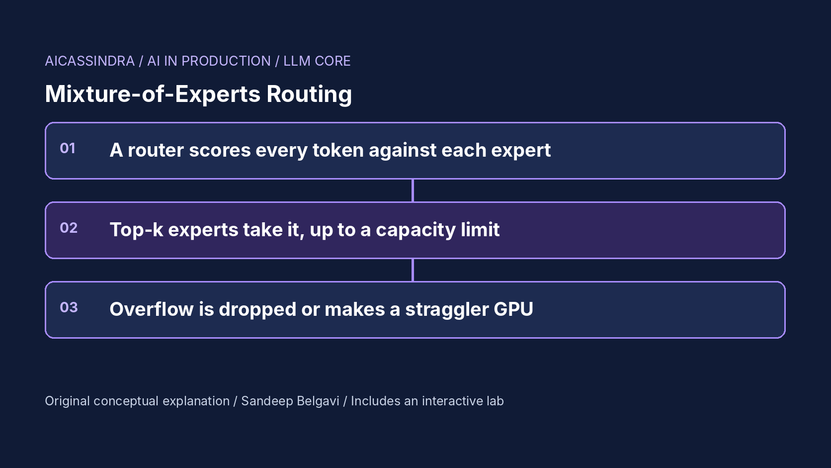
Mixture-of-experts (MoE) models promise the quality of a large model at the per-token compute of a small one: each token visits only a few of many expert feed-forward blocks. The promise holds only if the router spreads tokens sensibly. When it does not, one of two things happens. Either tokens that overflow an expert's fixed capacity are silently dropped, or, in dropless implementations, the GPU hosting the busiest expert becomes the straggler that every other GPU waits for.
This guide covers the mechanism from first principles: how top-k gating works, how capacity is computed and why tokens get dropped, how auxiliary losses and bias-based balancing keep the load even, and what all this means when you serve an MoE model with expert parallelism. It includes the arithmetic of capacity, the probability that small decode batches still touch every expert, the knobs in Megatron-Core, Hugging Face and vLLM, and the failure signatures to watch. The embedded lab runs a synthetic router on synthetic tokens so you can watch drops, imbalance and rerouting change together.
The router in one paragraph
An MoE layer replaces a transformer block's single feed-forward network with E expert networks and a router. The router is usually a single linear layer: for each token's hidden state x, it computes a score for every expert, s_e = x · w_e, applies a softmax, and selects the top k experts. The token is sent to those experts, and their outputs are combined using the gate weights (often renormalised over the selected k). Only k of E experts run per token, so compute per token scales with k while parameter count scales with E.
Shazeer and colleagues introduced the sparsely gated MoE layer in 2017 with noisy top-k gating. GShard scaled it with top-2 routing, Switch Transformer simplified to top-1, and recent open models use designs such as 8 experts with top-2 (Mixtral 8x7B) or many fine-grained experts with a larger k plus shared experts that every token visits (DeepSeek-V3 uses 256 routed experts with 8 active per token and one shared expert). The router's weights are learned with the rest of the model, which is the source of both its usefulness and its instability: nothing in the plain language-modelling loss tells it to spread the load.
Capacity: where dropped tokens come from
Hardware likes fixed shapes. Classic MoE implementations allocate a fixed buffer per expert, called its capacity, and compute it from the batch:
capacity = ceil(capacity_factor x tokens_per_batch x k / num_experts)

# lab default: 2,048 tokens, top-2, 16 experts
capacity_factor 1.00 -> ceil(1.00 x 2048 x 2 / 16) = 256 slots per expert
capacity_factor 1.25 -> 320 slots per expert (20% of all slots are spare)
capacity_factor 2.00 -> 512 slots per expert (at least 50% spare)

for each (token, expert) assignment in router order:
    if load[expert] < capacity: load[expert] += 1      # processed
    else: dropped += 1                                  # skips the expert
With a capacity factor of 1.0, capacity equals the perfectly even share. Any imbalance at all means some expert overflows. Overflowing assignments are dropped: the token skips that expert and its representation continues through the residual connection unchanged. With top-2, a token that loses one expert still gets the other; a token that loses both gets no expert computation at that layer.
Raising the capacity factor reduces drops but every extra slot is padding that costs compute and memory on every batch whether or not tokens fill it. Switch Transformer reported good results with capacity factors in the range of 1.0 to 1.25 when combined with load balancing, and found that higher factors trade speed for fewer drops. In the lab, mission one starts at factor 1.0 with no balancing, where roughly one assignment in ten is dropped.
Load balancing: auxiliary losses and bias terms
Because the language-modelling loss alone rewards a router that sends everything to whichever experts happen to be ahead early in training, MoE training adds pressure toward even load. The classic form, used in Switch Transformer, is an auxiliary loss:
aux_loss = alpha x E x sum over experts of ( f_e x P_e )
  f_e = fraction of tokens whose top choice is expert e   (not differentiable)
  P_e = mean router probability assigned to expert e      (differentiable)
  alpha ~ 0.01 in the Switch paper; minimised when both are uniform at 1/E
ST-MoE added a router z-loss that penalises large router logits, which improved training stability. Both losses fight the main objective a little: too high a coefficient forces tokens away from the experts that suit them. DeepSeek-V3 took a different route, called auxiliary-loss-free balancing: each expert has a bias added to its routing score only for the purpose of selecting the top k, and after each step the bias of overloaded experts is decreased and the bias of underloaded experts increased by a small step gamma. Gate weights still come from the original scores, so the bias steers traffic without distorting the mixture.
The lab implements this bias rule. The γ slider is the update step, applied after every batch over 24 warm-up batches. Small γ cannot catch up with a strong skew; large γ balances quickly but reroutes many tokens away from their preferred expert, which the lab's quality proxy charges for.
Why balance matters even when nothing is dropped
Modern training and inference stacks increasingly run MoE dropless: kernels such as those in MegaBlocks handle variable numbers of tokens per expert with block-sparse or grouped matrix multiplications, so there is no capacity and nothing is dropped. Imbalance then shows up as time instead of quality. With expert parallelism, experts are spread across GPUs; each batch, tokens are sent to their experts' GPUs with an all-to-all exchange, processed, and sent back. The layer finishes when the slowest GPU finishes.
If the busiest expert receives 1.6 times its fair share and sits on a GPU whose other experts are not correspondingly idle, that GPU carries the most work and every other GPU waits. In the lab's illustrative cost model, the MoE layer time is a fixed part plus the busiest GPU's token count times a per-token cost plus an all-to-all term. Switching the default setup from capacity mode to dropless removes all drops but raises layer time from about 4.4 ms to about 5.0 ms, because the straggler GPU now processes every token it received. Balancing brings it back down.
| Mode | What imbalance costs | What you watch |
|---|---|---|
| Capacity with drops | Quality: skipped expert computation | Drop rate per layer, per expert |
| Capacity, high factor | Compute and memory on padding | Share of empty slots |
| Dropless | Latency: straggler GPU | Max-to-mean expert load, per-GPU time |
Decode batches: small, noisy, and memory-bound
During generation, each decode step routes only as many tokens as there are running sequences, perhaps 32 to 256. Per-expert counts are then very noisy. With 128 tokens, top-2 and 16 experts, the even share is 16 tokens; ordinary randomness gives some experts 25 or more in a step even with a well-balanced router. A capacity factor that was safe for 2,048-token training batches drops tokens at decode time, which is why serving stacks generally avoid token dropping. Mission three asks you to fix exactly this case.
Small batches also change the memory arithmetic. A decode step is memory-bound, and an MoE step reads the weights of every expert that received at least one token. The probability that a given expert receives nothing from a batch of B tokens is roughly (1 - k/E)^B:
E = 8,  k = 2,  B = 16  -> (0.75)^16  = 0.010  -> ~99% of experts are read
E = 64, k = 4,  B = 16  -> (0.9375)^16 = 0.356 -> ~64% of experts are read
E = 64, k = 4,  B = 128 -> (0.9375)^128 ~ 0.0003 -> essentially all experts read
So at realistic batch sizes, an MoE decode step reads close to all of its expert weights, even though each token only uses a few. MoE saves compute per token, but the whole model must be resident in GPU memory and much of it is streamed every step. Size serving memory and bandwidth for total parameters, not active parameters.
The knobs in real systems
Names differ between frameworks; the questions are the same. Treat the table as a map, and check the exact flags for your version.
| Concept | Where you meet it | Notes |
|---|---|---|
| Experts and top-k | Model config, for example num_local_experts and num_experts_per_tok in Hugging Face Mixtral configs | Fixed by the checkpoint; do not change at serving time |
| Aux loss coefficient | router_aux_loss_coef (Transformers), --moe-aux-loss-coeff (Megatron-Core) | Training-time only; matters when you fine-tune |
| Capacity factor and drop policy | --moe-expert-capacity-factor, --moe-token-drop-policy (Megatron-Core) | Unset capacity usually means dropless |
| Expert parallelism | --enable-expert-parallel in recent vLLM versions; SGLang and TensorRT-LLM have equivalents | Changes which GPU becomes the straggler |
| Router z-loss | --moe-z-loss-coeff (Megatron-Core) | Stability, not balance |
Fine-tuning deserves special care. A fine-tune on a narrow dataset can skew the router toward a few experts, the router equivalent of overfitting, unless the balancing loss is kept on during fine-tuning. If you fine-tune MoE models, log per-expert token counts for every layer as a standard training metric, and compare them before and after. The lab's hot experts event models a router that comes back from a fine-tune favouring two experts; mission two asks you to rebalance it without buying more capacity.
Choosing experts, k and routing style
Most teams inherit E and k with the checkpoint, but they matter when you compare models or train your own. More, smaller experts with a larger k (fine-grained MoE) give the router more combinations to choose from and smooth out the load statistically, because each token's work is split into more pieces. The cost is more routing decisions, more all-to-all traffic and more small matrix multiplications, which can be less efficient on GPUs. Shared experts, which every token visits regardless of routing, absorb common knowledge so routed experts can specialise; they also give every token a guaranteed path even if a routed assignment is dropped.
Top-1 routing, as in Switch Transformer, halves routing compute and communication relative to top-2, but a dropped assignment then means the token gets no expert at all at that layer, so top-1 is less forgiving of overflow. Expert-choice routing turns the problem around: each expert picks its top tokens up to a fixed capacity, which guarantees perfect balance by construction, but some tokens may be chosen by no expert and others by several, and the scheme does not map naturally onto autoregressive decoding where tokens arrive one step at a time. For serving, token-choice routing with dropless kernels is the common pattern today; check what your chosen model and engine actually implement.
Testing a routing change safely
Routing behaviour is easy to change by accident: a new fine-tune, a different quantisation of the router weights, a change in expert-parallel layout or a new traffic mix can all move it. A safe rollout compares the old and new configurations on the same replayed traffic and reports four numbers per MoE layer: the share of assignments dropped (if any), the max-to-mean expert load, the per-GPU MoE time spread, and task quality on your evaluation set. Look at the worst layer, not the average; imbalance often concentrates in a few layers.
Quantisation deserves a specific mention. Router logits are small differences between large dot products, and aggressive quantisation of the router can flip top-k choices for tokens near a decision boundary. Many quantisation recipes keep the router in higher precision for that reason. If you quantise an MoE model, compare the routing decisions of the quantised and original models on the same inputs and report the share that changed.
A worked example: Belgavi's Book Store traffic shift
Imagine the hypothetical Belgavi's Book Store serves an MoE model with 16 experts, top-2, spread over 8 GPUs. Most days, questions spread across many topics. Then a seasonal promotion makes 62% of all tokens come from one topic: questions about a single book series. Experts that specialise in that kind of text receive far more than their share.
With a capacity factor of 1.0, the lab drops about 27% of assignments under the shift, and the quality proxy falls to about 84. Switching to dropless removes drops, but the busiest expert now carries about three times the mean load and the layer time rises from roughly 4.4 to 6.2 ms (all values calculated by the lab's illustrative model). Turning on bias balancing with a small step brings the busiest expert down and the layer time back to about 5.1 to 5.3 ms, at the cost of rerouting about a fifth of tokens away from their first-choice expert. Push γ much higher and the load looks perfectly even, but so many tokens are rerouted that the quality proxy drops below the target. Mission four asks you to find that narrow band.
The lesson generalises: balance is not a single number to maximise. It is a trade between specialisation and hardware efficiency, and the right point depends on traffic that can change overnight.
Failure modes and how to detect them
- Silent token dropping. Quality drifts down with no error. Export per-layer drop rates if your stack uses capacity, and alert on any increase.
- Straggler GPUs. In dropless expert-parallel serving, one GPU's utilisation runs consistently higher than the others while latency rises. Per-GPU timing and per-expert token counts reveal it.
- Router collapse during fine-tuning. A few experts take most tokens. Log the max-to-mean expert load per layer during training.
- Traffic-dependent imbalance. A model balanced on general text can be unbalanced on your domain. Measure routing statistics on a replay of production traffic, not on a benchmark.
- Sizing for active parameters. Planning GPU memory from active parameters leads to out-of-memory errors at load time; all experts must be resident.
Common mistakes include copying a capacity factor from a training recipe into a setting with much smaller batches, treating the auxiliary loss coefficient as free to raise, and reading uniform expert loads as proof of a healthy router when heavy balancing may be overriding its preferences.
Run the lab: Expert traffic control: route tokens without drops or stragglers
The lab routes synthetic tokens drawn from eight topics through a router whose experts loosely specialise in those topics. Bars show how many assignments each expert received in the last batch: the kept part in blue, overflow beyond capacity in red. Bands underneath group experts by GPU for expert parallelism. Start with mission one, where a capacity factor of 1.0 and no balancing drop about a tenth of all assignments.
Prefer a full-width view? Open the standalone lab. Your stars are saved in this browser and shown on the series hub.
What to do next
- Log per-expert token counts for every MoE layer on a replay of production traffic and compute the max-to-mean load.
- Find out whether your training and serving stacks drop tokens, and if so export per-layer drop rates as metrics.
- Size GPU memory and bandwidth for total parameters, not active parameters, and verify how many experts each decode step touches.
- If you fine-tune an MoE model, keep load balancing on and compare per-expert loads before and after.
- With expert parallelism, measure per-GPU MoE time to find stragglers instead of relying on average utilisation.
- Re-check routing statistics after major traffic mix changes, such as a new product line or language.
Sources and further reading
- Outrageously Large Neural Networks: The Sparsely-Gated Mixture-of-Experts Layer (Shazeer et al., 2017)
- Switch Transformers: Scaling to Trillion Parameter Models with Simple and Efficient Sparsity (Fedus et al.)
- ST-MoE: Designing Stable and Transferable Sparse Expert Models (Zoph et al., 2022)
- MegaBlocks: Efficient Sparse Training with Mixture-of-Experts (Gale et al., 2022)
- DeepSeek-V3 Technical Report (auxiliary-loss-free load balancing)
- Mixtral of Experts (Jiang et al., 2024)
Related in this series:
- Tensor or Pipeline Parallelism for Serving: Choosing How to Split a Model
- Grouped-Query Attention: How Sharing KV Heads Shrinks Inference Memory
- Compute-Optimal Model Sizing: Applying Chinchilla Scaling Laws to a Real Budget
Diagrams, examples and the lab model are original educational material. Lab numbers are calculated by a synthetic model, not measured on real hardware or services.
Views are my own and do not represent any employer, past or present.