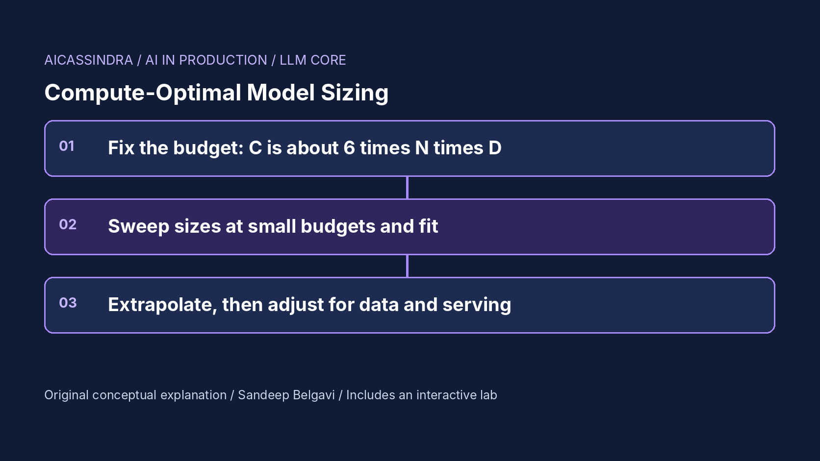
Every pretraining or continued-pretraining project eventually turns into one question: we have this many GPU-hours, so how big should the model be and how many tokens should it see? Get it wrong in one direction and you train a large model on too little data; in the other, a small model saturates while you keep paying for tokens it can barely use. Both are expensive in a way that no amount of later fine-tuning recovers.
This guide works through the compute-optimal answer from the Chinchilla scaling-law work, with the arithmetic to apply it to a real budget: FLOPs from GPU-hours, the loss surface, IsoFLOP pilot runs, and the roughly 20 tokens per parameter rule that falls out. It then covers the three situations where the compute-optimal answer is the wrong answer for production: when serving cost dominates, when unique data runs out, and when your pilot runs are too noisy to trust. The embedded lab lets you make each decision on a synthetic loss surface.
From GPU-hours to FLOPs
Training a dense transformer costs about six floating-point operations per parameter per token: roughly two for the forward pass and four for the backward pass. With N parameters and D training tokens, total training compute is C ≈ 6 N D. That approximation ignores attention's dependence on sequence length and some smaller terms, but for models of a few billion parameters and up at ordinary context lengths it is close enough to plan with.
The budget you control is usually GPU-hours, not FLOPs. Converting needs the hardware's peak throughput and the fraction of it your training stack actually achieves, model FLOPs utilisation (MFU):
C = GPU_hours * 3600 * peak_FLOPs * MFU

example (illustrative):
  500,000 H100-hours * 3600 s * 989e12 FLOP/s (dense BF16 peak) * 0.40 MFU
  = 7.1e23 FLOPs

a 70B model at that budget can see  D = C / (6 N) = 7.1e23 / (6 * 70e9) = 1.7e12 tokens
MFU is the number most often over-assumed. Well-tuned large runs have reported figures in the 40 to 50% range; 30 to 40% is common, and a stack with slow interconnect, frequent checkpoint stalls or restarts can do worse. Planning at 50% and achieving 30% means your real budget is 40% smaller, which changes the optimal model size. Measure MFU on a short run of the real configuration before you size the model, and include expected downtime in the GPU-hours you plan with.
The loss surface and the Chinchilla result
The Chinchilla paper trained more than 400 models from 70M to over 16B parameters on 5B to 500B tokens and modelled final pretraining loss as a function of both:
L(N, D) = E + A / N^alpha + B / D^beta

E        : irreducible loss of the data distribution
A/N^alpha: shortfall from finite model size
B/D^beta : shortfall from finite training data
Minimising L subject to 6ND = C gives power laws for the optimal size and data, N_opt ∝ C^a and D_opt ∝ C^b with a + b = 1. Chinchilla's three estimation approaches put both exponents near 0.5: parameters and tokens should grow in equal proportion as compute grows. That overturned the earlier Kaplan et al. recommendation, which put much more of each extra unit of compute into parameters. The practical summary that spread was about 20 training tokens per parameter. The headline demonstration was a 70B model trained on 1.4T tokens that outperformed the 280B Gopher model trained on 300B tokens with about the same compute.
One caveat matters if you reuse the published coefficients. A 2024 replication attempt found that the parametric fit (approach 3) as reported was inconsistent with the paper's other two approaches and implied an implausibly narrow confidence interval; refitting on data reconstructed from the paper gave coefficients consistent with roughly 20 tokens per parameter. The lab uses those refitted coefficients. Neither set transfers exactly to your data, tokenizer or architecture, which is why the next section matters more than the constants.
IsoFLOP pilots: measure your own optimum
Rather than trusting someone else's coefficients, run your own small experiments. The IsoFLOP method (Chinchilla's approach 2) is the most direct: pick a few small compute budgets, and at each budget train several model sizes, each for exactly the number of tokens that budget allows. Final loss against log model size traces a valley; fit a parabola, and its minimum is the compute-optimal size for that budget. Fit a straight line through those minima on log-log axes, and extrapolate to your target budget.
import numpy as np
minima = []
for C_pilot, runs in pilot_runs.items():          # runs: list of (N, final_loss)
    x = np.log10([n for n, _ in runs]); y = np.array([l for _, l in runs])
    a, b, c = np.polyfit(x, y, 2)                   # parabola in log N
    if a > 0:
        minima.append((np.log10(C_pilot), -b / (2 * a)))
cx, nx = np.array(minima).T
slope, intercept = np.polyfit(cx, nx, 1)            # log N_opt = slope * log C + intercept
N_opt_target = 10 ** (slope * np.log10(C_target) + intercept)
Two practical points. First, the valley is flat near the bottom, which is good news for production (being somewhat off costs little) and bad news for estimation (noise in a single run can move the fitted minimum a long way). Each pilot run's loss is noisy because of data order, initialisation and learning-rate schedule details; small runs are noisier. More runs per budget, sizes spread evenly on both sides of the minimum, and the same learning-rate schedule shape scaled to each run's length all help. Second, pilots cost compute. Three budgets at 1/3,000, 1/1,000 and 1/300 of the target with five runs each spend about 2.3% of the target budget, a reasonable insurance premium for a decision that fixes the rest.
How flat is flat? Thinking in wasted compute
Loss differences between nearby model sizes look tiny, often in the third decimal place, which makes them easy to dismiss. A more useful way to read them is compute-equivalent waste: how much compute would a correctly sized model need to reach the same loss? With the lab's coefficients at about 7e23 FLOPs, the following figures are calculated, not measured:
| Model size | Tokens per parameter | Loss | Budget effectively wasted |
|---|---|---|---|
| 8B | ~1,900 | 2.02 | ~82% |
| 20B | ~300 | 1.99 | ~48% |
| 40B | ~75 | 1.97 | ~16% |
| 70B | ~24 | 1.97 | under 1% |
| 280B | ~1.5 | 1.98 | ~42% |
Within a factor of about 1.5 of the optimum in either direction the waste is a few per cent; at a factor of four it is around half the budget. The 280B row is the Gopher-style mistake: a model too large for its budget, starved of data. The 20B and 8B rows are not necessarily mistakes, as the next section shows; they are what you choose deliberately when the model will be served at scale.
When to train past the optimum: serving cost
Compute-optimal means the lowest loss for a fixed training budget. It says nothing about what the model costs afterwards. Generating a token costs about 2N FLOPs, so a model's lifetime inference compute is roughly 2 N T for T served tokens. For a model that will serve hundreds of billions of tokens a day, that quickly dwarfs training. The rational objective becomes training cost plus serving cost at a target quality, and the answer is a smaller model trained on far more than 20 tokens per parameter. Work on inference-aware scaling laws formalises this, and widely used open models are trained this way: several 7B to 8B models have been trained on 2T to over 15T tokens, hundreds or thousands of tokens per parameter.
A concrete, illustrative case using the lab's model: a 70B model trained compute-optimally for 500k H100-hours ($1.25M at an assumed $2.50 per GPU-hour) and then serving 200 trillion tokens at an assumed 30% FLOP utilisation needs about 2.6e7 GPU-hours to serve, roughly $66M. A 12.6B model trained for 1M GPU-hours reaches a slightly worse but acceptable loss and costs about $2.5M to train and $12M to serve. The serving assumption is crude (decode is usually memory-bandwidth bound, and batching, quantization and hardware all move it), but the direction is robust: once lifetime serving tokens are many times training tokens, shrink the model and train it longer. Mission three in the lab asks you to find that point.
When data runs out: repetition and the data wall
The scaling laws assume every training token is fresh. For general web-scale pretraining at moderate size that is roughly true; for a domain model (a single language, a codebase, a specialist corpus) or at the largest budgets, it is not. Repeating data is worth less than new data, but not worthless: a study of data-constrained scaling found that a few epochs of repetition were almost as good as unique data, with value decaying after that and approaching zero after many tens of epochs. Their fit models repeated tokens as an exponentially decaying contribution with a characteristic scale of about fifteen repetitions; check the paper before reusing the constants.
The consequence for sizing is that tokens become relatively more expensive than parameters, so the optimum shifts toward a larger model trained for fewer effective tokens than the unconstrained rule says. With the lab's settings and only 0.15T unique tokens, the optimum moves from about 80B to about 105B parameters. The alternative levers are to get more data (filtering less aggressively, adding related domains, synthetic data with care) or to reduce the budget, because past a point extra compute buys very little.
Turning the decision into a run configuration
Once N and D are chosen, the token count has to be expressed in the trainer's own units, and the learning-rate schedule has to match it. Most frameworks count steps or samples, not tokens:
| Quantity | Megatron-LM style flags | Hugging Face Trainer style |
|---|---|---|
| Tokens per step | --global-batch-size × --seq-length | per-device batch × devices × gradient_accumulation_steps × sequence length |
| Run length | --train-iters or --train-samples | max_steps |
| Schedule length | --lr-decay-iters / --lr-decay-style | lr_scheduler_type, warmup_steps |
For example, 1.7T tokens at a global batch of 1,024 sequences of 4,096 tokens is about 4.2M tokens per step and roughly 405,000 steps. Flag names differ between versions and forks, so check the documentation of the release you run. Two details from the scaling-law work matter here. The Chinchilla authors observed that a cosine schedule whose length greatly exceeds the actual number of training steps gives worse final loss, so pilot runs must each use a schedule sized to their own length, or the IsoFLOP valley is biased toward small models. And the token count is the effective count after any packing, filtering and deduplication, so measure it from the data loader rather than from raw corpus size.
A worked example: Belgavi's Book Store
Suppose the hypothetical Belgavi's Book Store plans continued pretraining of a base model on book metadata, reviews and catalogue text, with a fixed allocation of 100,000 GPU-hours at a measured 38% MFU. That is about 100,000 × 3,600 × 989e12 × 0.38 ≈ 1.35e23 FLOPs. Ignoring the starting checkpoint, the 20-tokens-per-parameter rule suggests N ≈ sqrt(C / 120) ≈ 34B parameters and about 0.67T tokens.
Three facts change that. The shop's corpus has about 60B unique tokens, so 0.67T would mean eleven passes: a data wall. The assistant built on the model is expected to serve about 5T tokens a year, which favours a smaller model. And continued pretraining starts from an existing model, so the from-scratch law is only a guide. The team runs IsoFLOP pilots on their own data at 1/1,000 and 1/300 of the budget, sees a flat valley between 3B and 8B for those budgets once repetition is accounted for, and chooses an 8B base trained on about two passes over the corpus plus a share of general data to limit forgetting. All numbers here are illustrative; the procedure is the point.
Failure modes and how the lab maps to them
The common mistakes are: sizing from an assumed MFU instead of a measured one; reusing published coefficients across a different tokenizer, data mix or architecture; extrapolating from pilot runs at a single budget, or with all pilot sizes on one side of the minimum; tuning learning rate and schedule for one size and reusing them for all, which biases the valley; ignoring serving cost when the model will be deployed at scale; and ignoring repetition when the data is limited. Detection is mostly a matter of honesty in the pilots: plot every IsoFLOP curve, check that each has a visible minimum, and report the uncertainty of the extrapolation, not just the point estimate.
In the lab, mission one starts with a Gopher-style model far too large for its budget. Mission two adds a data wall and asks you to move the size in the direction the repetition penalty requires. Mission three switches on heavy serving and asks for a quality target at the lowest total cost, which pulls in the opposite direction. Mission four makes the pilot runs noisy and asks for an extrapolation you can trust while spending little on pilots.
Run the lab: Spend the budget: size a model with IsoFLOP curves
The left chart shows the predicted final loss for every model size at your training budget (an IsoFLOP curve), the true optimum in green, the size your pilot runs predict in pink, and your chosen size as the moving dot. The right chart shows the pilot runs at three small budgets with their fitted parabolas; white circles mark each fitted minimum. Start with the default 20B model, find the bottom of the valley, then load mission one.
Prefer a full-width view? Open the standalone lab. Your stars are saved in this browser and shown on the series hub.
What to do next
- Measure MFU on a short run of your actual training configuration and convert your GPU-hour budget to FLOPs with it.
- Run IsoFLOP pilots at three or more small budgets on your own data, with sizes on both sides of the expected minimum, and plot every curve.
- Report the extrapolated optimal size with an uncertainty range, and re-fit if any pilot curve lacks a clear minimum.
- Count unique tokens in your corpus and compute how many passes the planned run implies; adjust the size if it exceeds a few epochs.
- Estimate lifetime serving tokens and add inference cost (about 2N FLOPs per token) to the sizing decision before fixing N.
- Record the chosen N, D, budget, MFU and the reasoning in the run plan so later continued-pretraining decisions start from it.
Sources and further reading
- Training Compute-Optimal Large Language Models (Chinchilla)
- Scaling Laws for Neural Language Models
- Chinchilla Scaling: A replication attempt
- Scaling Data-Constrained Language Models
- Beyond Chinchilla-Optimal: Accounting for Inference in Language Model Scaling Laws
Related in this series:
- Mixture-of-Experts Routing: Load Balancing, Capacity Factors and Dropped Tokens
- LoRA Rank, Alpha and Target Modules: Choosing Settings That Actually Work
- Why INT4 Breaks Some Layers: Outliers, Group Size and Activation-Aware Scaling
Diagrams, examples and the lab model are original educational material. Lab numbers are calculated by a synthetic model, not measured on real hardware or services.
Views are my own and do not represent any employer, past or present.