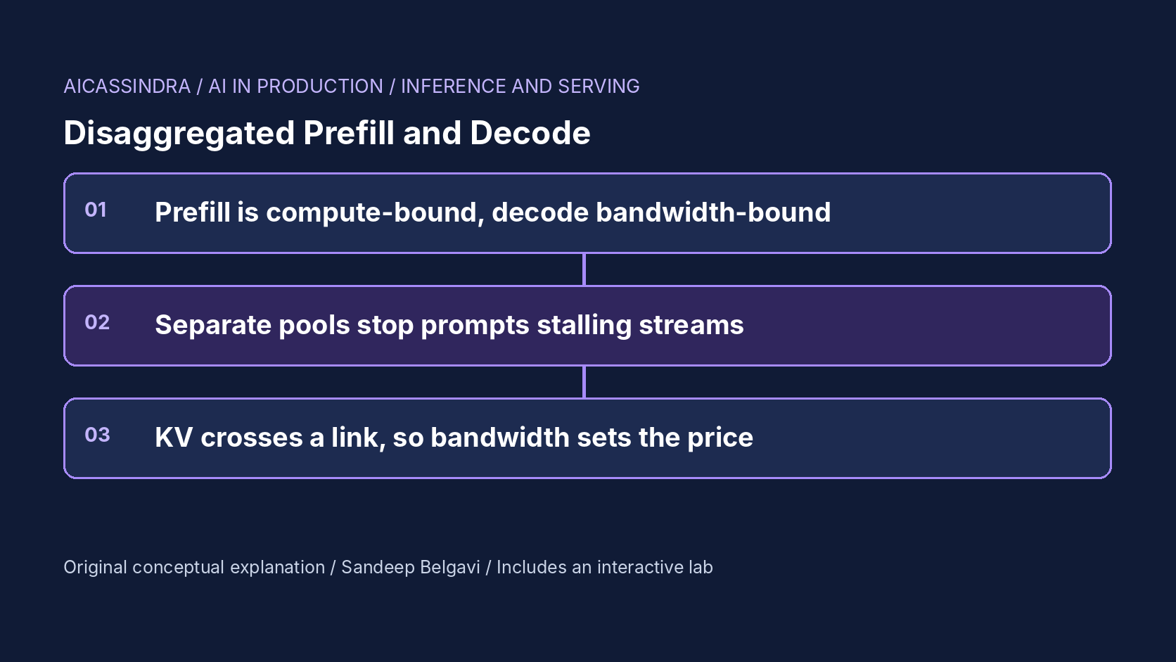
Every LLM request has two phases with opposite personalities. Prefill reads the whole prompt in one large, parallel forward pass and is limited by compute. Decode produces one token per step for each sequence and is limited by memory bandwidth. A conventional server runs both on the same GPUs, inside the same batches, and that is where the trouble starts: a long prompt arriving on a GPU makes every stream on that GPU wait while it is prefilled.
Disaggregated serving puts the two phases on different GPU pools. Prefill GPUs process prompts and build the KV cache, the cache is shipped over an interconnect, and decode GPUs generate the rest of the answer without ever being interrupted by a prompt. The idea was developed in systems such as DistServe, Splitwise and Mooncake, and is now available in open-source serving stacks. It is not free: you pay in KV transfer bandwidth, in a second scaling problem (the ratio between pools), and in operational complexity. This guide works through when the split pays, with the arithmetic for interference, transfer cost and pool sizing, and the lab lets you run a synthetic fleet both ways.
Two phases, two bottlenecks
Prefill multiplies a matrix of prompt-token activations by every weight matrix. With thousands of tokens in flight, the arithmetic intensity is high and the GPU's tensor cores are the limit; doubling the prompt roughly doubles the time. Decode multiplies a single new token per sequence by the same weights, so each step streams all the weights and the KV cache from memory to do very little arithmetic. Its cost is dominated by bytes moved, which is why batching many sequences per step is what makes decode efficient.
The two phases also want different things from parallelism and batching. Prefill latency (and therefore time to first token, TTFT) improves with more GPUs per instance via tensor parallelism; decode throughput improves with larger batches and more memory for KV. The SLOs differ too: TTFT for prefill, time per output token (TPOT) for decode. When both phases share one instance, one configuration has to serve two masters.
# lab constants (illustrative, not measured)
prefill:  0.05 ms per prompt token     -> 20,000 prompt tokens/s per GPU
decode:   8 ms + 0.25 ms per sequence + 0.00004 ms per context token, per step

one 2,500-token prompt prefilled inside a decode step:
  extra time = 2,500 * 0.05 = 125 ms
  every stream on that GPU sees a 125+ ms gap between two tokens
  against a 25 ms TPOT target, that single step costs five tokens' worth of budget
Interference: why colocation hurts at load
The continuous batching guide in this series explained iteration-level scheduling. Here is its uncomfortable side. A colocated GPU that admits a new request runs that request's prefill in the next step, together with the decodes of everything already running. At low load this happens rarely and nobody notices. As load rises, admissions happen on a larger share of steps, and each one stretches the step for all running sequences.
Do the arithmetic for one GPU receiving 3 requests per second with 2,500-token prompts. Prefill takes 3 × 125 = 375 ms of every second, so more than a third of wall time is spent in steps that contain a prefill. A request that decodes for 220 tokens over a few seconds will be interrupted by several of these stalls, and its average TPOT rises sharply even though its own decode steps would have taken 12 to 20 ms. That is the regime mission one starts in: four colocated GPUs at 12 requests per second, p99 inter-token gap above 200 ms, and only 87% of requests meeting both SLOs.
Chunked prefill, covered in its own guide, is the colocated answer: split each prompt into bounded slices so each step does a limited amount of prefill work. It reduces the size of each stall but not the total prefill work sharing the decode GPU. Disaggregation removes the sharing entirely. Many deployments use both: chunked prefill inside the prefill pool to bound its own latency, and a split to protect decode.
What it costs to move the KV cache
Splitting the phases means the KV cache built by prefill must reach the decode GPU before the second token can be produced. Its size is fixed by the model:
| Model shape (FP16 KV) | KV per token | 2,000-token prompt | At 12.5 GB/s | At 50 GB/s | At 300 GB/s |
|---|---|---|---|---|---|
| 8B-class, 32 layers, 8 KV heads × 128 | 128 KiB | 250 MiB | about 21 ms | about 5 ms | under 1 ms |
| 70B-class, 80 layers, 8 KV heads × 128 | 320 KiB | 625 MiB | about 52 ms | about 13 ms | about 2 ms |
These are calculated from the formula 2 × layers × KV heads × head dimension × 2 bytes, ignoring protocol overhead. The rough bandwidth classes are 100 Gb Ethernet (12.5 GB/s), a 400 Gb RDMA NIC (50 GB/s) and NVLink-class links inside a node (hundreds of GB/s). Two conclusions follow. With RDMA or NVLink, transfer time is small next to prefill time for the same prompt, so it barely moves TTFT. Over ordinary Ethernet, transfer can rival prefill for large models and long prompts, and it queues when many prompts finish at once. Real implementations overlap transfer with prefill layer by layer and stream KV as it is produced, which hides some of the cost; the lab charges it after prefill completes, which is the pessimistic case.
Transfers also need somewhere to land. The decode GPU must have free KV memory for the incoming sequence, so the decode pool's KV capacity, not just its compute, bounds how many requests can be in flight. Systems such as Mooncake go further and build a distributed KV store across CPU memory and SSD so that prefill output and cached prefixes can be fetched by whichever decode node needs them.
Sizing the two pools
With separate pools you now have two capacity problems. The prefill pool must keep up with prompt tokens per second; the decode pool must keep up with output tokens per second at a batch size whose step time meets the TPOT target. A first estimate needs only averages:
prefill GPUs  >= rate * mean_prompt_tokens / prefill_tokens_per_s_per_gpu / target_utilisation
decode GPUs   >= rate * mean_output_tokens / decode_tokens_per_s_per_gpu_at_SLO_batch

# mission two, lab constants
rate 22 req/s, prompt 2,000, output 220
prefill: 22 * 2000 = 44,000 tok/s / 20,000 per GPU = 2.2 -> 3 GPUs
decode : 22 * 220  =  4,840 tok/s; a GPU at ~24-step-ms with ~40 sequences
         produces ~1,650 tok/s within a 25 ms TPOT -> 3 GPUs
The ratio depends on the workload, not the hardware alone. Long prompts with short answers (document question answering, classification with reasoning, RAG) are prefill-heavy and want more prefill GPUs; short prompts with long answers (chat, code generation, reports) are decode-heavy. Mission four's long-document surge ends with five prefill GPUs for three decode GPUs, while a chat workload might run one prefill GPU for every four or five decode GPUs. The ratio also moves during the day as the traffic mix shifts, which is why production systems scale the two pools independently and some can reassign instances between roles.
The failure signature of a wrong ratio is easy to read once you know it. If the prefill pool is saturated, TTFT rises while TPOT stays flat and decode GPUs sit partly idle. If the decode pool is saturated, TPOT rises (or requests wait for decode admission and TTFT rises too, if you count the first token at decode) while prefill GPUs idle. Mission two starts with six prefill and two decode GPUs: the decode pool drowns and goodput falls to about 13%, with three quarters of the fleet doing almost nothing.
Goodput is the metric that settles it
Throughput alone hides the problem disaggregation solves. A colocated GPU can post excellent tokens per second while half its requests miss the TPOT target. DistServe argued for goodput: the rate of requests that meet both their TTFT and TPOT SLOs, and per-GPU goodput as the cost metric. The lab reports the share of requests meeting TTFT ≤ 1.5 s and per-request TPOT ≤ 25 ms, and good requests per second per GPU.
Framed this way, the decision is concrete. Colocation wins when prompts are short, load is modest, or SLOs are loose: there is no transfer cost and no pool to balance, and no GPU idles while the other phase is busy. Disaggregation wins when long prompts and tight TPOT targets coexist at high load, because then colocated GPUs must be run at low utilisation to keep stalls rare. In the lab, mission four shows it directly: colocated serving needs ten GPUs to keep 95% goodput through the long-document surge, while a disaggregated fleet does it on eight.
The knobs in real systems
Disaggregated serving is moving quickly, so treat these as places to look rather than settled flags, and check your version's documentation:
| System | How the split is configured | KV transport |
|---|---|---|
| vLLM | Separate prefill and decode instances with a KV transfer configuration (--kv-transfer-config) naming a connector and each instance's role | Pluggable connectors, for example NIXL or LMCache based |
| SGLang | --disaggregation-mode prefill or decode per server, plus a router in front | Selectable transfer backend, for example Mooncake or NIXL |
| NVIDIA Dynamo | Orchestrates prefill and decode workers on top of engines such as vLLM, SGLang or TensorRT-LLM | NIXL |
| TensorRT-LLM | Context (prefill) and generation (decode) executors as separate servers | Built-in KV cache transceiver |
Whatever the stack, the decisions are the same: how many prefill and decode instances, which parallelism each uses, whether the first token is emitted by the prefill or the decode side (which changes what TTFT includes), what happens when the decode pool cannot accept a transfer, and which network path the KV takes. Placing a prefill and decode pair inside one NVLink domain keeps transfers fast; spreading them across racks puts them on the data-centre network.
Failure modes and how to see them
- Link saturation. KV transfer time climbs and TTFT (if counted at decode) follows, while both pools look underused. Export transfer latency and bytes per second per link. Mission three degrades the link to one eighth: with 4,000-token prompts, each request ships about 500 MB and transfers queue for seconds. The incident answer is to stop shipping KV over the slow path, by falling back to colocated serving or keeping pairs within one fast domain, not to wait for a network upgrade.
- Wrong pool ratio after a traffic shift. One pool's utilisation pegs while the other's falls. Alert on the ratio of prefill to decode utilisation, not just each one.
- Decode-side KV exhaustion. Transfers wait for free blocks on the decode GPU, and preemption there forces re-transfer or recompute. Watch decode KV usage and admission wait.
- Prefill head-of-line blocking. One 30,000-token prompt monopolises a prefill instance. Use chunked prefill or route very long prompts to dedicated instances.
- Measuring TTFT inconsistently. If the prefill node emits the first token, TTFT excludes transfer and the second token absorbs it. Compare configurations with the same definition. The lab counts the first token when the decode pool emits it, after the transfer.
A worked example: document answers for Belgavi's Book Store
The hypothetical Belgavi's Book Store adds a feature that answers questions about long catalogue documents: prompts average 4,000 tokens, answers 220, and traffic peaks at 6 requests per second. Product wants TTFT under 1.5 s and smooth streaming at 25 ms per token. Using the lab's constants, prefill demand is 6 × 4,000 = 24,000 tokens per second, a little over one GPU's worth; decode demand is about 1,300 tokens per second, comfortably one GPU at a batch size that keeps steps under 25 ms. A two-plus-two disaggregated layout leaves headroom on both sides.
The KV for each request is 4,000 × 128 KiB, about 500 MB. Over 50 GB/s RDMA that is 10 ms, negligible. Over shared 100 Gb Ethernet it is about 40 ms, still acceptable alone, but the 6 transfers per second now occupy about a quarter of the link, and at one eighth of its bandwidth during an incident transfers take about a third of a second each and queue behind each other. The team therefore keeps prefill and decode workers paired in the same node, and keeps a colocated configuration ready as the fallback. These figures are calculated with illustrative constants; the procedure, not the numbers, is what transfers to a real deployment.
Common mistakes
- Disaggregating a short-prompt chat workload, where interference is small and the split mostly adds transfer cost and a second pool to size.
- Sizing the pools from average traffic and never revisiting the ratio as the prompt-length mix changes.
- Benchmarking with a fixed prompt length, which hides the interaction between long prompts and tight TPOT targets that motivates the split.
- Ignoring the network path: KV crossing a congested shared network in production behaves nothing like the benchmark on one node.
- Comparing colocated and disaggregated configurations on throughput instead of goodput per GPU.
Run the lab: Split the fleet: prefill pool, decode pool, and the link between
The lab simulates sixty seconds of synthetic requests on a small GPU fleet, with every GPU running on its own clock. Colocated GPUs mix whole-prompt prefills into their decode steps; in the disaggregated layout, prefill GPUs batch prompts, the KV cache crosses a link of the chosen bandwidth, and decode GPUs only decode. The canvas scrolls through 2.5 seconds of each GPU's timeline: blue steps decode, amber bars are prefill batches, and red marks colocated steps that blew through the TPOT target. Start colocated, then work through the missions.
Prefer a full-width view? Open the standalone lab. Your stars are saved in this browser and shown on the series hub.
What to do next
- Plot p99 inter-token gap against prompt length on your current fleet; a strong correlation means prefill interference is costing you.
- Compute KV bytes per request for your models and typical prompts, and compare transfer time on your actual network path with prefill time.
- Report goodput (share of requests meeting both TTFT and TPOT SLOs) and goodput per GPU alongside throughput.
- Estimate the prefill-to-decode ratio from prompt and output token rates, then confirm it with a load test that replays your real length mix.
- Try chunked prefill first on colocated serving and measure how much of the interference it removes before taking on a split.
- If you disaggregate, alert on transfer latency, per-pool utilisation imbalance and decode-side KV usage, and keep a tested colocated fallback.
Sources and further reading
- DistServe: Disaggregating Prefill and Decoding for Goodput-optimized Large Language Model Serving (OSDI 2024)
- Splitwise: Efficient Generative LLM Inference Using Phase Splitting (ISCA 2024)
- Mooncake: A KVCache-centric Disaggregated Architecture for LLM Serving
- Taming Throughput-Latency Tradeoff in LLM Inference with Sarathi-Serve (OSDI 2024)
- NVIDIA Dynamo (GitHub)
Related in this series:
- Chunked Prefill: Stopping Long Prompts From Freezing Every Other Stream
- TTFT, TPOT and Goodput: Setting LLM Latency SLOs That Mean Something
- Continuous Batching Explained: Why Static Batches Leave GPUs Idle
Diagrams, examples and the lab model are original educational material. Lab numbers are calculated by a synthetic model, not measured on real hardware or services.
Views are my own and do not represent any employer, past or present.